Flow Field Analysis of a Turbulent Channel Controlled by Scalloped Riblets

Introduction

Drag reduction is of great importance because of the environmental and economic benefits from the reduced fuel consumption [1]. As one of the oldest and most investigated drag reduction methods, riblets, small protruding surfaces along the direction of the flow, had been known to be capable of reducing friction drag up to 8% with appropriate height and spacing in spite of the extra surface area. Early experiments conducted by Walsh et al. [2, 3], Bacher et al. [4], and Bechert et al. [5] tested different shapes including triangular, rectangular (or blade), trapezoidal, semi-circular, and other shape grooves with various sizes to get an optimal drag reduction rate. Experiments on concave and convex riblet shapes showed that drag reduction increases as the peak curvature increases, or as the radius of valley curvature increases, which means that an optimum riblet shape should have sharp peaks and curved valleys [2]. However, later investigations put more emphasis on the riblet tip rather than the valley, arguing that the tip sharpness plays an important role in damping the spanwise velocity fluctuations and thus limiting the momentum transport and turbulence intensity.

Two drag reduction regimes of riblets had been recognized [5], i.e., the “viscous regime,” $W^{+}<10-15$, where the drag reduction rate increases almost linearly with the riblet width; and the “breakdown regime,” $W^{+}>15-20$, where the drag reduction rate reaches a maximum and then decreases even to the point of drag increase. Here, $W^{+}$ represent the riblet width in wall units and the protruding surfaces would be referred to as roughness when entering the drag increase state. The physical mechanisms for drag reduction by riblets have been extensively studied, for example Walsh [6], Choi et al. [7], Choi [8], and Rstegari et al. [9]. Researchers often owe the credit to the interaction between the riblet surfaces and the longitudinal vortices of the turbulent boundary layer. One widely accepted explanation for riblets of the viscous regime, or for infinitesimal riblets, relies heavily on the concept of protrusion height [10, 11]. Intuitively, the protrusion height is understood as the distance between the riblet tip plane and the origin of the velocity profile, which lies between the riblet tip and riblet valley. The idea behind the emphasis of the protrusion height concept is that the influence of riblets is mainly constrained to within the inner layer and is thus viewed as an inner layer control strategy, and what the outer layer can “feel” is just the shear between the inner and outer layer. Therefore, the protrusion height denotes the location of a hypothetical flat plane that the outer layer perceives. The true protrusion height definition was given by Luchini et al. [11] From the intuitive definition above, we can easily define a longitudinal protrusion height $h_{\parallel }$ and a perpendicular protrusion height $h_{\perp }$ based on average streamwise and spanwise velocity respectively. Then the difference $∆h=h_{\parallel }-h_{\perp }$ is referred to as the protrusion height. The basic idea is that compared with streamwise flow, $∆h$ represents the extent at which the cross-flow fluctuations are hampered, which had been viewed as critical for the turbulence generation cycle. In the viscous regime, the drag reduction rate is linearly dependent on this protrusion height $∆h$, a fact that has been verified by experiments and numerical simulations for various riblet shapes. However, the mechanism for the deterioration of drag reduction, or the “breakdown regime” remains controversial. The generation of secondary streamwise vortices by unsteady crossflow separation, which brings high speed flow towards the riblet surfaces, was suggested by Goldstein and Tuan [12], but secondary streamwise vortices do not necessarily lead to drag increase. For example, spanwise oscillation of the wall can also decrease drag [13, 14]. The second group of theories emphasized the scale interaction between riblet surfaces and turbulent coherent structures, i.e., near-wall streaks and streamwise vortices [7, 15]. Generally, the optimal lateral scale of riblets is an order of magnitude smaller than the spacing between low-speed streaks (about 100 in wall units). It was argued that for riblets larger than $W^{+}\approx 20-30$, the near wall streamwise vortices could move freely and lodge inside the riblet valleys, which leads to an increase of wall surface area exposed to the sweep motion induced by those vortices. On the other hand, for smaller riblets, the streamwise vortices would stay above the riblet tips, and only the tip region could be subjected to the induced sweeps. Alternatively, Garcia-Mayoral and Jimenez [16] attributed the breakdown to the appearance of large-scale spanwise rollers. The mechanisms suggest plausible reasons based on experimental and numerical observations, but lack substantial support of improved design of riblets based on these theories.

As a bio-inspired technique mimicking the denticles of fast swim sharks, riblets are possibly the only turbulent drag reduction strategy that have been tested in application. Szodruch [17] reported that covering of riblets on 70% of the surface on an Airbus 320 commercial airplane leads to a 2% reduction in oil consumption. Instances of using riblets in sports, for example, on the hulls of boats and the surfaces of racing swimsuits, have been successful [18]. In contrast to the canonical arrangement, novel riblet concepts have been introduced. Nugroho et al. [19] explored the possibility of using ordered and directional surfaces to redirect the near wall flow. Benhamza et al. numerically investigated variable spacing riblets of rectangular shape in turbulent channel flows. Riblets with a sinusoidal variation along the streamwise direction [20, 21] had also been devised to mimic the spanwise oscillation strategy to reduce drag, however, these gained very little further drag reduction. Boomsma [22] numerically studied denticles resembles sharkskin in turbulent boundary layer, however, obtained drag increase instead of drag reduction. These expeditions generally failed to surpass the optimum drag reduction rate of conventional riblets, indicating a lack of full understanding of the drag reduction mechanism.

The plausible mechanisms of breakdown imply a requirement of tip sharpness of riblet for high drag reduction performance. However, sharp tips pose challenges for manufacturing and maintenance. Actually, Walsh [2] experimentally found that the optimum riblet appears to have sharp peaks and significant valley curvature. Launder and Li [23] also reported that the U-form (or scalloped) riblets can achieve a superior performance to the corresponding V-shaped riblets with the same height and width. Based on the protrusion height concept and numerical simulation of riblet controlled boundary layer transition, Wang et al. [24] showed that scalloped riblets could have better performance than corresponding triangular riblets with sharper tips. The scalloped riblet shape we considered is constructed by smoothly connecting two third-order polynomials.

where $W$ is the width of the riblet, and the shape of the other half riblet ($W/2<z\le W$) can be obtained by symmetry about $z=W/2$. Note, we have selected a coordinate system consistent with the following three-dimensional simulations. $x$, $y$, and $z$ directions are streamwise, wall-normal, and spanwise directions respectively. Being aligned in the streamwise direction, $x$ is not present in the riblet shape definition. $\gamma$ is the height-width ratio while $A$ and $B$ are chosen parameters to determine the curvature at the tip and valley of the riblets. Note that an extra factor of $2$ is introduced to make $A$ and $B$ the coefficients of second order terms when the width of the riblet is $S=1$ and height-width ratio is $\gamma =0.5$. $a$, $b$, and $z^{*}$ are obtained by requiring the two polynomials smoothly connected, i.e., the functions value, first and second derivatives are continuous at $z^{*}$. Despite the non-linearity in $z^{*}$, the equations can be solved analytically

To guarantee that $z^{*}/W$ is in the range of $\left(\mathrm{0,0.5}\right)$, we have to ensure that the given A and B satisfies

An extreme exists with $A=B=6$, when the two polynomials are identical and the curvatures at the tip and valley are perfectly balanced. Thus, Eq. 1 represents a system of scalloped riblets, the tip and valley curvatures of which can be easily defined. Wang et al. [24] calculated the protrusion heights for scalloped riblets with various $A$, $B$, and $\gamma$ values with a boundary element algorithm proposed by Luchini et al. [11], and found that for a larger height-width ratio $\gamma$, the protrusion height is mainly determined by $A$, i.e., the curvature at riblet tip, while for a smaller height-width ratio $\gamma$, the protrusion height is mostly dependent on $B$, i.e., the curvature at the riblet valley. However, for riblets in practical applications, the height-width ratio is generally in the range of $0.5\le \gamma \le 1.2$, the protrusion height is influenced equally by $A$ and $B$. Therefore, the shape of the riblet valley cannot be overlooked, and should be designed more carefully. It is also illustrated by direct numerical simulations of a boundary layer transition that a scalloped riblet, which is not as sharp in the tip as a corresponding triangular riblet with the same height-width ratio, nevertheless has a larger drag reduction rate, which is in accordance with protrusion height results. Another advantage of the scalloped riblet over the triangular riblet is its stronger resilience to riblet tip erosion, which means better manufacturing and maintenance performances. For the current study, we will focus on the same scalloped riblet as in Wang et al. [24] with $A=25$, $B=1.6$ and $\gamma =0.5$. It was obtained, to four decimal digits, that $a=100.6970$, $b=-1.4793$ and $z^{*}/W=0.0940$. Note that similar groove shapes had been studied by Klumpp et al. [25] for boundary layer transition but without detailed information of the groove shape. In addition, there are two methodologies to resolve the riblet shapes in numerical simulations, which involve the utilization of either body-fitted meshes or an immersed boundary method. With body-fitted meshes, the riblet shapes are better represented, but lack the versability of representing different shapes and sharp corners, especially when high-order numerical methods are adopted. On the other hand, the immerse boundary method can easily be used to simulate different riblet shapes even with the same mesh, which, however, has been criticized for low accuracy near the wall surfaces. For the current study, we choose the immersed boundary method for its versability and adopt Lagrange interpolation [26] to improve the accuracy near the wall surface.

One important aspect in understanding the flow dynamics is the identification of vortices. Noted by Küchemann [27], vortices are the “sinews and muscles of the flow.” However, no consensus on the definition of vortices has been reached. Popular methods including $Q$, $\Delta$, ${\lambda }_2$, ${\lambda }_{ci}$, $\mathrm{\Omega }$ [28–32] and other criteria have been introduced to visualize vortices in various flows. However, these methods mainly suffer from two issues: 1) These methods are different with different physical reasoning and dimension units among each other; 2) as scalar-valued methods, no directional information about the rotational motion is provided. To overcome these issues, a new vortex vector, Liutex vector [33, 34], was introduced with its magnitude as twice the angular velocity of the rigid rotation part of the fluid motion and its direction as the local rotational axis. An explicit expression for the Liutex vector $\mathit{R}$ in terms of vorticity $\mathit{\omega }$, eigenvalues and eigenvectors of the velocity gradient tensor is proposed by Wang et al. [35] which leads to efficiency improvement and physical intuitive comprehension as

where ${\lambda }_{ci}$ is the imaginary part of the complex conjugate eigenvalues and $\mathit{r}$ is the real eigenvector of velocity gradient tensor. Thereafter, multiple vortex identification methodologies have been developed including the Liutex iso-surfaces, Liutex-$\mathrm{\Omega }$ method [36, 37], Liutex core line method [38, 39], objective Liutex method [40], etc. In addition, a particular feature of the Liutex vector is that it is free from shear contamination. Kolář and Šístek [41] found that only the Liutex vector is not contaminated by stretching and shear in that an arbitrary adding or subtracting of stretching and shear would not alter the resulting vortex identification. This distinctive feature has been utilized by Ding et al. [42] to develop a new Liutex-based sub-grid model for large eddy simulation, which has been proved to outperform the famous Smagorinsky model in homogeneous isotropic turbulence and turbulent channel flows. In the current study, the Liutex vortex identification method will be adopted to analyze the flow field of riblet controlled turbulent channels.

The paper is organized as follows. Section Numerical Methods and Case Setup introduced the numerical methods adopted, especially the customized immersed boundary method that we use to model riblet surfaces. Section Numerical Results presents the numerical results, discussing the drag reduction rate, mean flow and turbulent statistics, premultiplied power spectrum density, and instantaneous flow field, with particular attention paid to the Liutex field. Finally, conclusions are drawn in Section Conclusion.

Numerical Methods and Case Setup

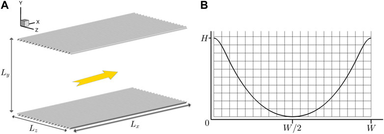
The canonical case of a turbulent channel flow at Reynolds number ${Re}_{\tau }=180$ was considered and used to study the drag reduction capacity of the scalloped riblets. The open-source finite difference software “Incompact3d” [43, 44] was adopted to simulate the flat plate and riblet channels, with which the incompressible Navier-Stokes equations were numerically solved. Periodic conditions were naturally employed in the streamwise ($x$) and spanwise ($z$) direction, whilst no-slip conditions were applied in the upper and lower walls in the wall normal direction ($y$). For the riblet case, the no-slip condition was implemented with the immersed boundary method (IBM) which will be elaborated in the following. Sixth order compact schemes were adopted for spatial derivatives and a low-storage third-order Runge-Kutta scheme was used for time advancement. The pressure Poisson equation was solved with a pseudo-spectral method to ensure divergence-free condition up to machinery accuracy. The lengths for the computational domain were selected to be $L_x=4h$, $L_y=2h$ and $L_z=2h$ with $h$ as the half channel height. The domain is generally smaller compared to other direct numerical simulations of turbulent channel at ${Re}_{\tau }=180$, but still sufficient to capture all the length scales and meanwhile limits the overall mesh point number to accelerate the simulations. A schematic of the flow with riblets is shown in Figure 1A. Both meshes for the two cases were identical and include $256\times 129\times 360$ grid points in the streamwise, wall normal, and spanwise directions respectively. Uniform grids were used in the streamwise and spanwise directions, whilst a stretching grid was used in the normal direction with points clustered towards the wall surfaces. In wall units, the intervals in the streamwise and spanwise directions were ${∆x}^{+}\approx 2.81$ and ${∆z}^{+}\approx 1.00$ while the first interval adjacent to the wall was ${∆y}^{+}\approx 0.98$. Normally, this resolution is more than sufficient to resolve all the scales in channel flow, especially in the spanwise direction. With 18 riblets arranged spanwise, 20 mesh points were used to resolve one riblet, and the riblet width in wall units was $W^{+}=20$, which was around the optimum width. The distribution of mesh points near one riblet surface is shown in Figure 1B. The flow rate was kept constant every time step and the bulk velocity $u_b$ was thus kept as $2/3$ with a bulk Reynolds number of 2800. Note that the bulk Reynolds number was exact while the friction Reynolds number was only approximately 180 and the wall unit lengths in the current study were all obtained based on ${Re}_{\tau }=180$ unless otherwise stated.

FIGURE 1. (A) Sketch of the computational domain; (B) The mesh around the riblet surface.

The riblet surfaces were modeled with a customized immersed boundary method in “Incompact3d” based on an alternating direction forcing to ensure a no-slip boundary condition at the wall of the solid body [26]. A particular treatment was that no-zero velocities were set inside the solid body when computing derivatives to avoid discontinuities of the velocity field, which, of course, would not be used when outputting numerical results. Because the technique is important for both correctly resolving the riblet wall surfaces and precisely calculating the friction drag, which is certainly critical especially when aiming for about 5∼10 percent drag reduction, the procedure is described in more detail in the following.

For the adopted compact finite difference scheme, the derivatives along a directional line, which could cover both fluid and solid regions, were calculated simultaneously in a so-called implicit manner by solving systems of linear algebraic equations. If the condition of velocity component $u_i=0$ was to be set everywhere inside the solid domain, then the spatial derivative at the interfaces between fluid and solid would not be ensured to be continuous, which leads to deterioration of the solution. The problem only has a minor impact for low-order numerical scheme. When combined with high-order schemes, however, spurious oscillations would be generated at the interfaces. To deal with this issue, non-zero values inside the solid domain were set based on Lagrange or cubic spline interpolation from points on and adjacent to the interfaces. This described 1D procedure was dealt with sequentially for the three dimensions, and hence the name “alternating direction.” For the riblet case, we selected Lagrange interpolation and two points from each fluid side of the interfaces to do interpolation. Note that the first adjacent fluid nodes near the interfaces were not included for stability reasons.

To calculate wall shear stresses on a riblet surface, velocity gradients need to be calculated on these surfaces, which are not necessarily on mesh nodes. To obtain velocity gradients, we carried out interpolation the same way as described above on one dimensional basis. Then we used a simple finite difference based on the interface point and an interpolated point about the local mesh size away. Once velocity gradients are obtained, the wall shear stress ${\tau }_w$ can be calculated by

where $V_{\parallel }$ is the velocity parallel to the wall surface, and $n$ is the normal direction to the wall surface. It is not obvious when calculating wall shear stresses on riblet surfaces than flat surfaces. For riblet surfaces, the normal direction is ${\left[\begin{array}{ccc}0& n_2& n_3\end{array}\right]}^T$, the partial derivative $\partial V_{\parallel }/\partial n$ can be computed by

Then, the drag can be expressed as a line integral (actually a surface integral, however we can simply take average in streamwise direction because of the homogeneity)

where $L$ is the length of the curved surface in the spanwise direction. Transforming the curve integral into coordinate integral we get

where $L_2$ and $L_3$ are the normal and spanwise extent of the riblet surfaces. Note before using Eq. 8 to integrate, riblet-wise average should be carried out and the symmetry of the riblet surface used first to make the integrand single-valued in the y direction. Finally, to be comparable to the flat plate case, the skin friction coefficient $c_f$ is defined as

where $u_b$ is the bulk velocity.

Numerical Results

Drag Reduction Rate

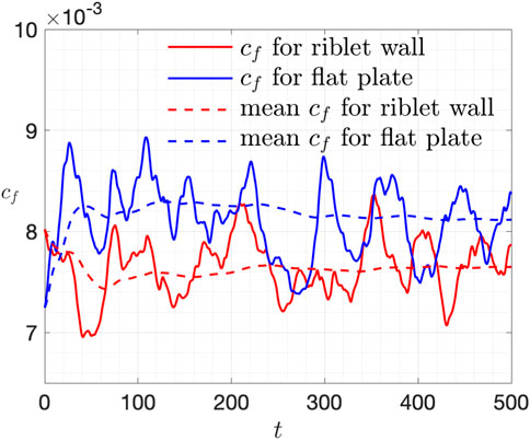
The initial condition for both cases with and without riblet control is interpolated from a direct numerical simulation of turbulent channel flow at ${Re}_{\tau }=180$ with a coarser grid and a larger computational domain. After the initial transient stage of 300 non-dimensional time units, with bulk velocity, $2/3$ of the fluids have flown through the computational domain 50 times, the friction coefficients are recorded for the following 500 time-units and are shown in Figure 2. Note that with the definition of skin friction coefficient $c_f$ presented in the last section, comparison of $c_f$ is equivalent to comparison of the total drag exerted on the whole wall surfaces. The cumulative averages of skin friction coefficients are also shown in Figure 2 with a clear drag reduction observed. The mean skin friction coefficients for flat plate and riblet wall are $8.12\times {10}^{-3}$ and $7.65\times {10}^{-3}$, which means the drag has been reduced by 5.77%. The friction Reynolds number is ${Re}_{\tau }=178.4$, slightly smaller than the nominal Reynolds number ${Re}_{\tau }=180$. Based on this actual Reynolds number, the width of the riblets in wall units is 19.8. We will continue to use wall units based on ${Re}_{\tau }=180$ in the following text. For corresponding triangular riblets with same width in wall units, and same height-width ratio, Walsh [3] reported a 2% drag reduction, while Choi [7] reported a 5% drag reduction. Similar settings for blade riblets in a larger Reynolds number of ${Re}_{\tau }=550$ result in a 4.45% drag reduction [45]. Generally, the current drag reduction rate of the scalloped riblet is higher than the corresponding triangular riblets with sharper tips. In addition, the scalloped tips are beneficial for the manufacturing and maintenance. The stochastic and intermittent behavior of the instantaneous skin friction coefficients come from the limited size of the computation domain and thus a small statistical sample. A simple Fourier analysis reveals that a peak exists for the frequency corresponding to a time period of $T=125$, which should be understood as a quantity related to the spatial scales in homogeneous directions. However, we will not make further discussions here.

FIGURE 2. Time history and cumulative mean of skin friction coefficients at both riblet and flat walls.

Mean Flow and Second-Order Statistics

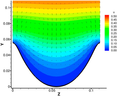
The streamwise, time-, and riblet-wise averaged flow field near a riblet is shown in Figure 3. First, it is clear that all three velocity components in the valley are quite small, which makes the skin friction on the valley surface of the riblet rather small. On the other hand, the mean streamwise velocity rapidly increases along the $y$ direction, creating high drag regions on the tips of the riblets. In addition, two secondary vortices can be found near the riblet tips, which has been reported by Choi et al. [7] and Wang et al. [35]. However, how such mean vortices correspond to instantaneous flow field remains unexplored.

FIGURE 3. Contours of mean streamwise velocity in the $y-z$ plane with in-plane velocity vectors.

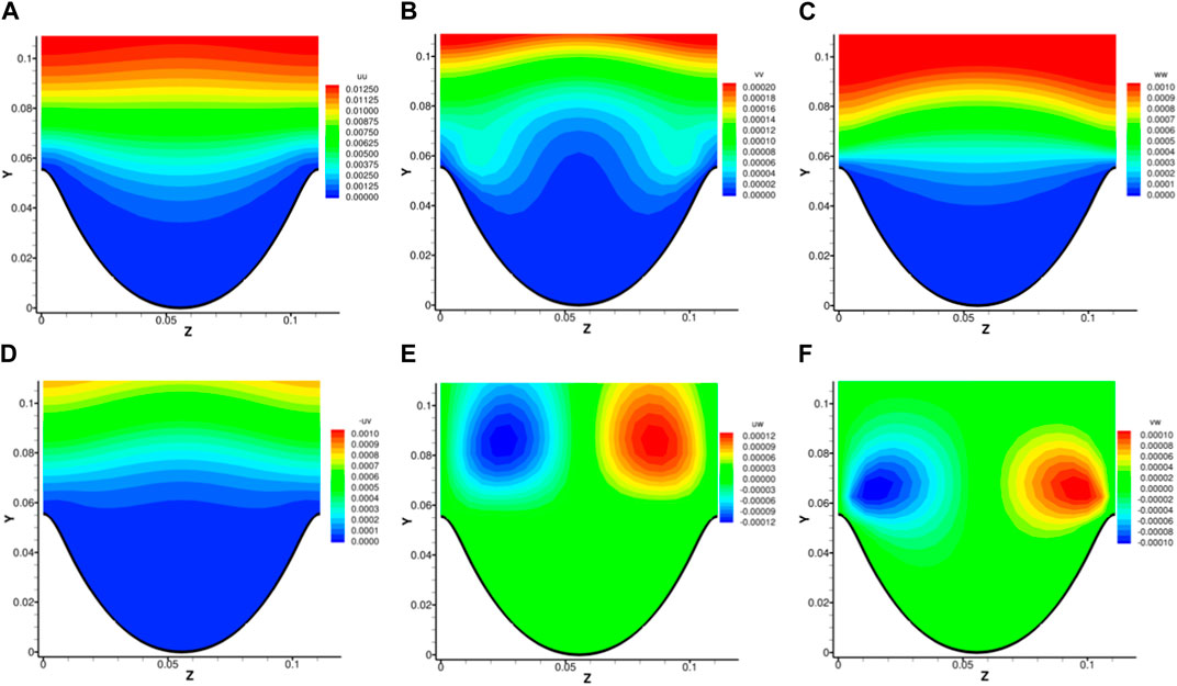
Figure 4 shows the Reynolds stresses near riblet surfaces with primes denoting fluctuations. It can be observed from the normal stresses in Figures 4A–C that fluctuations inside the riblet valley are quite small, and above $y\approx 0.11$ ($y^{+}\approx 20$ in wall units) the flow becomes almost uniform in the spanwise direction. This uniformity is in accordance with the assumptions of the viscous limit. Note the location of “W” shaped contour of $\overline{v^{\prime }{v}^{\prime }}$ is not the same as the mean secondary vortices. In addition, these fluctuations are superposed to the mean flow, and they cannot be created by these mean vortices. As shown in Figure 4D, $\overline{u^{\prime }{v}^{\prime }}$ is always negative near the riblet surface, which means a negative wall-normal fluctuation is accompanied by a positive streamwise fluctuations, and vice versa. In terms of quadrant analysis, more events happen in the second and forth quadrant of a $u’-v’$ plane, which are termed ejections and sweeps. Intuitively, a downward fluctuation brings high-speed flow towards the wall, thus creating a positive streamwise fluctuation, and an upward fluctuation brings low-speed flow away from the wall, creating a negative streamwise fluctuation. Different from Figures 4A–D, the green color in Figures 4E, F means no correlation between fluctuations. For the concentrations around $y=0.08$ in Figure 4E, we can see that for positive streamwise fluctuations, the correlated spanwise velocity would drive them towards the riblet tips, while for negative streamwise fluctuations, the correlated spanwise velocity would drive them to the top of the riblet valleys. This observation is in accordance with the average streamwise velocity in Figure 3. A similar situation can be observed for $\overline{v^{\prime }{w}^{\prime }}$ in Figure 4F. From the distributions of normal Reynolds stresses, we can see that the streamwise fluctuations are two-orders larger than that of the wall-normal and spanwise fluctuation, thus our interpretation of transport of streamwise fluctuations by spanwise fluctuations. On the other hand, the wall-normal and spanwise fluctuations are in the same order as shown in Figures 4B, C. Therefore, Figure 4F can also be interpreted as spanwise fluctuations towards riblet tips would be lifted up while spanwise fluctuations towards the top of the riblet valley tends to be pushed downwards. Another thing worth noting is that the concentrations of $\overline{u^{\prime }{w}^{\prime }}$ are located substantially higher than those of $\overline{v^{\prime }{w}^{\prime }}$. Those correlations cannot be accredited to a single or several vortices, if we view fluctuations as results of instantaneous vortices, but only a statistical average effect of many vortices.

FIGURE 4. Distributions of Reynolds stresses near riblet surfaces. (A) $\overline{u^{\prime }{u}^{\prime }}$, (B) $\overline{v^{\prime }{v}^{\prime }}$, (C) $\overline{w^{\prime }{w}^{\prime }}$, (D) $-\overline{u^{\prime }{v}^{\prime }}$, (E) $\overline{u^{\prime }{w}^{\prime }}$, (F) $\overline{v^{\prime }{w}^{\prime }}$.

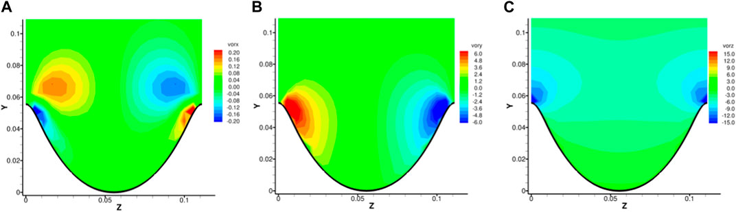
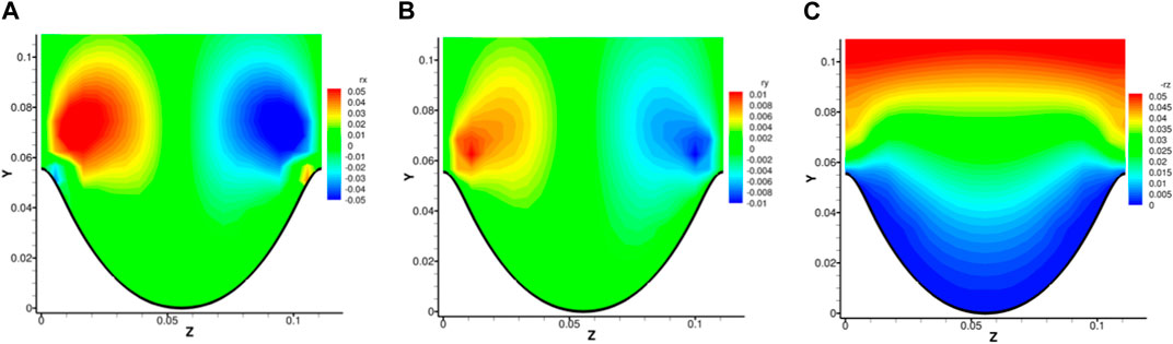
The distribution of mean vorticity and mean Liutex are shown in Figures 5, 6. We can see that for the spanwise and wall-normal components, the magnitude of vorticity components are two-orders larger than that of Liutex components. This is because besides Liutex-represented rotational motion, vorticity also contains pure shear, and contributions of high shears from $\partial u/\partial z$ and $\partial u/\partial y$ make the magnitude of vorticity components very large near the wall. A similar situation can be found for the streamwise component but with a smaller difference. This is because no background shear is present in the streamwise direction. Two mean streamwise vortices can be observed in accordance with the mean velocity field shown in Figure 3. In the vortex centers, it can be observed that Liutex takes up 50% of the vorticity magnitude, meaning the magnitude of Liutex is in balance with the magnitude of shear. Another observation is that, by no surprise, shears are closer to the wall while Liutex regions are located further away from the wall.

FIGURE 5. Distribution of mean vorticity near riblet surfaces. (A) $\overline{{\omega }_x}$, (B) $\overline{{\omega }_y}$, (C) $\overline{{\omega }_z}$.

FIGURE 6. Distribution of mean Liutex near riblet surfaces. (A) $\overline{R_x}$, (B) $\overline{R_y}$, (C) $\overline{R_z}$.

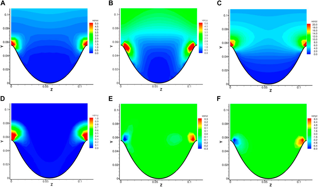
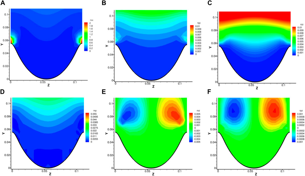
Second-order momentums of vorticity and Liutex components are shown in Figures 7, 8 respectively. The locations of concentrations of both $\overline{{\omega }_x^{\prime }{\omega }_x^{\prime }}$ and $\overline{R_x{R}_x}$ are on top of the tips of riblets but with different magnitude, indicating possible instantaneous streamwise vortices just above riblet tips, which we will verify in the following. As we noted above, shear is very large near the riblet tips in the spanwise and wall-normal direction. Therefore, the magnitude in the concentrations of $\overline{{\omega }_y^{\prime }{\omega }_y^{\prime }}$ and $\overline{{\omega }_z^{\prime }{\omega }_z^{\prime }}$ is substantially larger than that of $\overline{R_y{R}_y}$ and $\overline{R_z{R}_z}$. Note that we have used fluctuations denoted by prime for vorticity while using the original variable for Liutex, based on the idea that turbulence velocity fluctuations are created with the generations of multiple scale vortices. For example, a pure shear flow like a laminar boundary layer would have substantial spanwise vorticity near the wall, which from the Liutex system will all be classified as shear. Such shear would only affect the mean flow, but not the fluctuations. Thus, the fluctuations are assumed to come from the formation of vortices and the shears near the riblet tips acts as a bank for the rotational motion. The concentrations of both $\overline{{\omega }_y^{\prime }{\omega }_y^{\prime }}$ and $\overline{{\omega }_z^{\prime }{\omega }_z^{\prime }}$ disappear in the contours of $\overline{R_y{R}_y}$ and $\overline{R_z{R}_z}$ as shown in Figures 7B, C, 8B, C. There are no clear spanwise and wall-normal vortex patterns in the vicinity of riblet surfaces. For the cross-correlation terms, the strong correlation in $\overline{{\omega }_x^{\prime }{\omega }_y^{\prime }}$ in Figure 7D is not presented in Figure 8D, which means despite a high correlation of shear, the streamwise and wall-normal vortices are statistically decoupled above riblet tips. Similar for $\overline{{\omega }_x^{\prime }{\omega }_z^{\prime }}$ and $\overline{{\omega }_y^{\prime }{\omega }_z^{\prime }}$ as shown in Figures 7E, F, shear contributes mainly for the concentrations near riblet tips, while the correlation concentrations of $\overline{R_x{R}_z}$ and $\overline{R_y{R}_z}$ are well further away from the wall. An interesting observation is the similarities between the distributions of cross-correlations of Liutex components in Figures 8D–F and the distributions of shear Reynolds stresses shown in Figures 4D–F. Even though the concentration locations are shifted upward or downward a little bit for $x-z$ and $y-z$ correlations, the trend remains the same. As stated, the Liutex correlations are calculated using the original variable rather than fluctuations, which makes it easier to construct turbulence models based on the Liutex vector. Ding et al. [42] introduced a subgrid model for large eddy simulation based upon the eddy viscosity hypothesis. Non-isotropic models can also be easily formulated.

FIGURE 7. Distributions of second moments of vorticity near riblet surfaces. (A) $\overline{{\omega }_x^{\prime }{\omega }_x^{\prime }}$, (B) $\overline{{\omega }_y^{\prime }{\omega }_y^{\prime }}$, (C) $\overline{{\omega }_z^{\prime }{\omega }_z^{\prime }}$, (D) $-\overline{{\omega }_x^{\prime }{\omega }_y^{\prime }}$, (E) $\overline{{\omega }_x^{\prime }{\omega }_z^{\prime }}$, (F) $\overline{{\omega }_y^{\prime }{\omega }_z^{\prime }}$.

FIGURE 8. Distributions of second moments of Liutex components near riblet surfaces. (A) $\overline{R_x{R}_x}$, (B) $\overline{R_y{R}_y}$, (C) $\overline{R_z{R}_z}$, (D) $-\overline{R_x{R}_y}$, (E) $\overline{R_x{R}_z}$, (F) $\overline{R_y{R}_z}$.

Premultiplied Power Spectrum Density

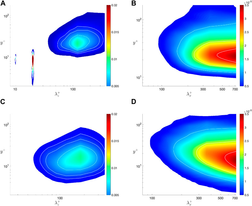
Contours of pre-multiplied energy spectra of flat plate channel and riblet controlled channel are shown in Figure 9. $k_x$ and $k_z$ are the streamwise and spanwise wavenumbers and ${\mathrm{\Phi }}_{uu}$ is the energy spectra of streamwise velocity fluctuations. It can be seen from Figure 9A that high energy regions can be found around wavenumber ${\lambda }_z^{+}=20$ and ${\lambda }_z^{+}=10$ at the height of $y^{+}=10$. Note that ${\lambda }_z^{+}=20$ corresponds to the width of the riblet while $y^{+}=10$ corresponds to the height of riblets. This is no surprise, as riblets enforce zero velocity inside the solid region and thus create periodic patterns at wavenumber ${\lambda }_z^{+}=20$. Harmonics includes ${\lambda }_z^{+}=10$, ${\lambda }_z^{+}=5$ and so on can be found in the pre-multiplied spectrum, but not shown in Figure 9A for wavenumbers less or equal to 5 because of their significance. On the other hand, the concentration of energy power spectra around $y^{+}=20$ represents the low-speed streaks, typical coherent structures found in wall bounded turbulence. These streaks had a typical spacing around 100 in wall units. However, compared to $k_z{\mathrm{\Phi }}_{uu}$ shown in Figure 9C for the flat plate channel, the spacing between the streaks decrease, which means that riblet, viewed as an inner-layer control method, also alters the buffer layer. The magnitude corresponding to the streaks remains basically the same. For the streamwise velocity component, the energy spectrum concentrates at a length scale equal to the length of the computational domain at the height of the buffer layer as shown in Figures 9B, D. In addition, the contours have been made more parallel to the streamwise direction by the riblet control, indicating a regulation of the flow field.

FIGURE 9. Contours of pre-multiplied energy spectra of channel flow with and without scalloped riblet surface: (A) $k_z{\mathrm{\Phi }}_{uu}$ with riblet surface; (B) $k_x{\mathrm{\Phi }}_{uu}$ with riblet surface; (C) $k_z{\mathrm{\Phi }}_{uu}$ without riblet surface; (D) $k_x{\mathrm{\Phi }}_{uu}$ without riblet surface.

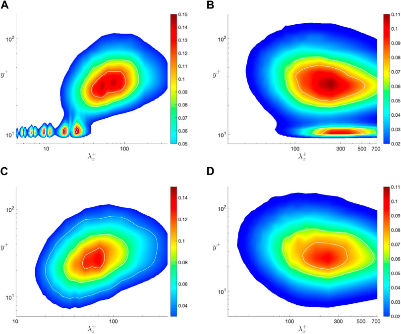
Low-speed streaks and streamwise vortices have been viewed as critical in the turbulence generation cycle. Here we adopt the Liutex methodology and use its streamwise component to represent streamwise vortices. The pre-multiplied energy spectra of $R_x$ with and without riblet control is shown in Figure 10. The situation is more complex for $R_x$ with riblet control above the height of riblets $y^{+}=10$ with a series of concentrations ranging from ${\lambda }_z^{+}=3$ to $25$ as shown in Figure 10A. It seems that those small concentrations appear in pairs, a pair around ${\lambda }_z^{+}=20$, then a pair around ${\lambda }_z^{+}=10$ and so on. It has been implied from Figure 8A that streamwise vortices exist just above the riblet tips. However, they are not always present for all riblet tips and they can be both negative and positive, which might be the reason for the energy spectrum pattern seen in Figure 10A. The larger scale at $y^{+}=40$ with riblet control is stronger than the scale at $y^{+}=30$ without riblet control. Note that, if we measure lengths in $y$ direction from the tip rather than the valley of the riblets, the heights at which the larger scale reside will be the same. In addition, we can see from Figure 10B that the streamwise vortices at the top of the riblet tips has a length scale of around ${\lambda }_x^{+}=200-300$, which our computational domain still can capture with $L_x^{+}=720$. The length scale is slightly larger than the length scale at $y^{+}=40$ with riblet control, which is stronger than that without riblet control as shown in Figure 10D. Overall, from the pre-multiplied energy spectra of $u$ and $R_x$, we can see that for the current riblet control, the statistical property changes are not limited to the viscous sublayer. The buffer layer and the bottom of the log layer are also affected by the riblet control. Spectra of $R_x$ more clearly shows the existence and influences of streamwise vortices just above the riblet tips, which we will further investigate in the following.

FIGURE 10. Contours of pre-multiplied energy spectra of channel flow with and without scalloped riblet surface: (A) $k_z{\mathrm{\Phi }}_{R_x{R}_x}$ with riblet surface; (B) $k_x{\mathrm{\Phi }}_{R_x{R}_x}$ with riblet surface; (C) $k_z{\mathrm{\Phi }}_{R_x{R}_x}$ without riblet surface; (D) $k_x{\mathrm{\Phi }}_{R_x{R}_x}$ without riblet surface.

Instantaneous Flow Field

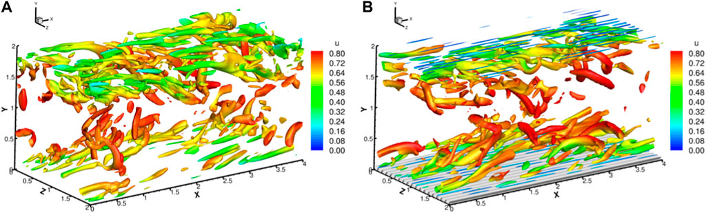
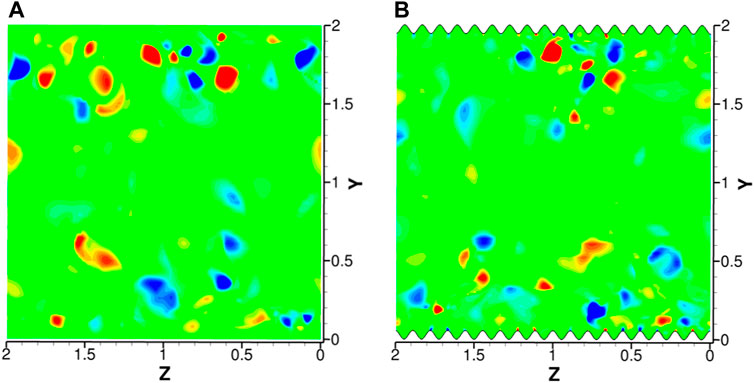
Instantaneous vortical structures are shown by iso-surfaces of Liutex magnitude $R=0.95$ for typical snapshots both with and without riblet control in Figure 11. Despite the chaotic appearance, streamwise vortices, hairpin and arc vortices, typical structures in a turbulent channel, can be observed in Figure 11A. The streamwise vortices just above the riblet tips that are mentioned above can be observed in Figure 11B. Note that we have removed the top riblet surface for visualization. Instantaneous contours of streamwise Liutex components at $x=2$ with and without riblets are shown in Figure 12. It can be seen that some riblet tips have those streamwise vortices, and some do not. In addition, the streamwise Liutex can be either positive or negative in a statistically balanced way. Therefore, they cannot be observed from the mean flow field as shown in Figure 3 and the mean vorticity and Liutex field as shown in Figures 5A, 6A. However, from the discussion above, those streamwise vortices should be very important in influencing the second-order moment statistics, and thus have a significant influence on the generation cycle of wall turbulence.

FIGURE 11. Instantaneous vortical structures visualized by iso-surfaces of Liutex magnitude $R=0.95$ for (A) flat plate channel and (B) riblet-controlled channel.

FIGURE 12. Instantaneous contours of streamwise component of Liutex vector for flat plate case (A) and riblet case (B).

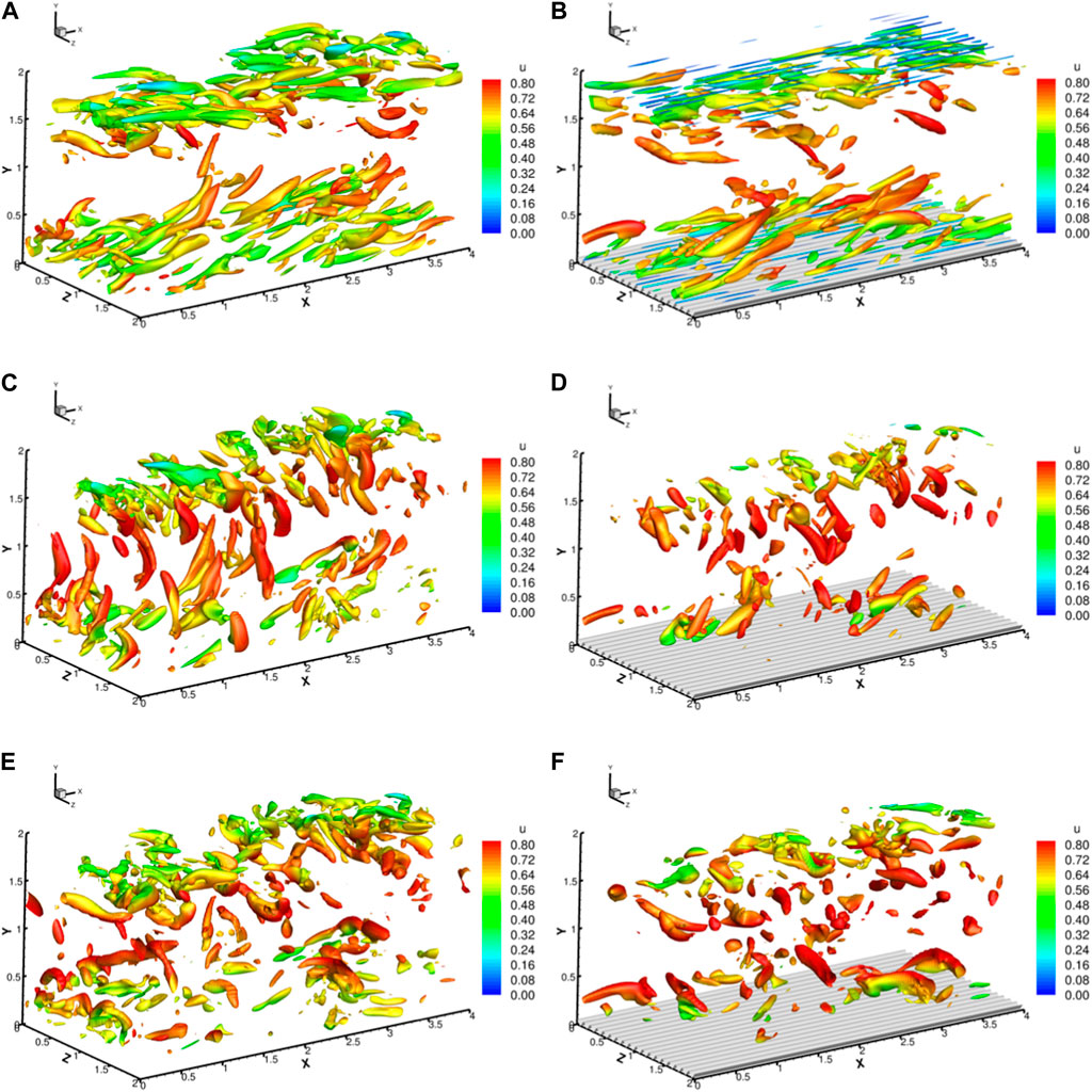
Figure 13 shows iso-surfaces of absolute values of Liutex components. It can be seen from Figures 13A, B that the streamwise vortices are located near the wall surfaces and it is reconfirmed that the vortices on the top of riblet tips are actually streamwise. For the snapshot shown in Figure 13C, multiple lengthy vortices in the $y$ direction can be observed, but for the riblet control case in Figure 13D, the y-direction vortices are lesser, and lack the directional arrangement. For iso-surfaces of $\left|R_z\right|$ in Figures 13E, F, we can find fewer structures in the riblet controlled case, and the structures tend to be more statistically isotropic. A visual inspection reveals possible weakening of spanwise and wall-normal vortices by riblet control.

FIGURE 13. Instantaneous iso-surfaces of absolute values of Liutex components for flat plate channel and riblet controlled channel. (A) $\left|R_x\right|=$ without riblets, (B) $\left|R_x\right|=$ with riblets, (C) $\left|R_y\right|=$ without riblets, (D) $\left|R_y\right|=$ with riblets, (E) $\left|R_z\right|=$ without riblets, (F) $\left|R_z\right|=$ with riblets.

Conclusion

We considered the kind of scalloped riblets constructed by smoothly connecting two third-order polynomials, and selected a scalloped riblet with shape parameters $A=25$ and $B=1.6$. The turbulent channel flows with and without riblet control were simulated with $W^{+}=20$, and height-width ratio $\gamma =0.5$. The drag reduction rate was 5.77%, which is generally larger than corresponding triangular riblets with sharper tips. The flow fields were then investigated carefully. Mean flow fields, Reynolds stress, correlations of vorticity and Liutex components, pre-multiplied spectra of streamwise velocity and Liutex component, and instantaneous flow fields were presented. It was found that streamwise vortices just above the riblet tips, which have a length scale of 200–300 in wall units, play a significant role in the controlling the flow field. Further investigations, especially the causal relations between those streamwise vortices and the drag reduction, should be analyzed. Moreover, it is imperative to consider the influence of the Reynolds number in the context of scalloped riblets, particularly in high Reynolds number flows, where the application of riblets for drag reduction is targeted.

Data Availability Statement

The data that support the findings of this study are available from the corresponding author upon reasonable request.

Author Contributions

HY: investigation; visualization; writing original draft. YH: review and editing. YW: conceptualization; investigation; methodology; code development; writing, editing of the manuscript. YQ: review and editing. SF: review and editing. All authors contributed to the article and approved the submitted version.

Funding

The current study is supported by Jiangsu Shuangchuang Project (JSSCTD202209), the National Science Foundation of China (Grant No. 12302312) and the National Science Foundation of the Jiangsu Higher Education Institutions of China (Grant No. 22KJB130011).

Conflict of Interest

The authors declare that the research was conducted in the absence of any commercial or financial relationships that could be construed as a potential conflict of interest.

References

1. Abbas, A, Bugeda, G, Ferrer, E, Fu, S, Periaux, J, Pons-Prats, J, et al. Drag Reduction via Turbulent Boundary Layer Flow Control. Sci China Technol Sci (2017) 60(9):1281–90. doi:10.1007/s11431-016-9013-6
CrossRef Full Text | Google Scholar
2. Walsh, M. Turbulent Boundary Layer Drag Reduction Using Riblets. In: 20th Aerospace Sciences Meeting; January 11-14, 1982; Orlando, Florida (1982).
4. Bacher, E, and Smith, C. A Combined Visualization-Anemometry Study of the Turbulent Drag Reducing Mechanisms of Triangular Micro-Groove Surface Modifications. In: Shear Flow Control Conference; March 12-14, 1985; Boul- der, Colorado (1985).
5. Bechert, DW, Bruse, M, Hage, W, Van Der Hoeven, JGT, and Hoppe, G. Experiments on Drag-Reducing Surfaces and Their Optimization with an Adjustable Geometry. J Fluid Mech (1997) 338:59–87. doi:10.1017/s0022112096004673
6. Walsh, MJ. Effect of Detailed Surface Geometry on Riblet Drag Reduction Performance. J Aircraft (1990) 27(6):572–3. doi:10.2514/3.25323
7. Choi, H, Moin, P, and Kim, J. Direct Numerical-Simulation of Turbulent-Flow over Riblets. J Fluid Mech (1993) 255:503–39. doi:10.1017/s0022112093002575
8. Choi, K-S. Near-Wall Structure of a Turbulent Boundary Layer with Riblets. J Fluid Mech (2006) 208:417–58. doi:10.1017/s0022112089002892
9. Rastegari, A, and Akhavan, R. The Common Mechanism of Turbulent Skin-Friction Drag Reduction with Superhydrophobic Longitudinal Microgrooves and Riblets. J Fluid Mech (2018) 838:68–104. doi:10.1017/jfm.2017.865
10. Bechert, DW, and Bartenwerfer, M. The Viscous-Flow on Surfaces with Longitudinal Ribs. J Fluid Mech (1989) 206:105–29. doi:10.1017/s0022112089002247
11. Luchini, P, Manzo, F, and Pozzi, A. Resistance of a Grooved Surface to Parallel Flow and Cross-Flow. J Fluid Mech Digital Archive (2006) 228:87. doi:10.1017/s0022112091002641
12. Goldstein, DB, and Tuan, TC. Secondary Flow Induced by Riblets. J Fluid Mech (1998) 363:115–51. doi:10.1017/s0022112098008921
13. Baron, A, and Quadrio, M. Turbulent Drag Reduction by Spanwise wall Oscillations. Appl Scientific Res (1995) 55(4):311–26. doi:10.1007/bf00856638
14. Jung, WJ, Mangiavacchi, N, and Akhavan, R. Suppression of Turbulence in Wall-Bounded Flows by High-Frequency Spanwise Oscillations. Phys Fluids A: Fluid Dyn (1992) 4(8):1605–7. doi:10.1063/1.858381
15. Suzuki, Y, and Kasagi, N. Turbulent Drag Reduction-Mechanism above a Riblet Surface. Aiaa J (1994) 32(9):1781–90. doi:10.2514/3.12174
16. GarcÍA-Mayoral, R, and JimÉNez, J. Hydrodynamic Stability and Breakdown of the Viscous Regime over Riblets. J Fluid Mech (2011) 678:317–47. doi:10.1017/jfm.2011.114
17. Szodruch, J. Viscous Drag Reduction on Transport Aircraft. In: 29th Aerospace Sciences Meeting; January 11-14, 1988; Reno, Nevada (1988).
Google Scholar
19. Stalio, E, and Nobile, E. Direct Numerical Simulation of Heat Transfer over Riblets. Int J Heat Fluid Flow (2003) 24(3):356–71. doi:10.1016/s0142-727x(03)00004-3
20. Peet, Y, Sagaut, P, and Charron, Y. Towards Large Eddy Simulations of Turbulent Drag Reduction Using Sinusoidal Riblets. In: Proceedings of the 5th IASME/WSEAS International Conference on Fluid Mechanics and Aerodynamics; August 25-27, 2007; Athens, Greece (2007).
21. Sasamori, M, Iihama, O, Mamor, H, Iwamoto, K, and Murata, A. Experimental and Numerical Studies on Optimal Shape of A Sinusoidal Riblet for Drag Reduction in Wall Turbulence. In: Ninth International Symposium on Turbulence and Shear Flow Phenomena; June 30 - July 3 (2015); Australia (2015).
22. Boomsma, A, and Sotiropoulos, F. Direct Numerical Simulation of Sharkskin Denticles in Turbulent Channel Flow. Phys Fluids (2016) 28(3). doi:10.1063/1.4942474
23. Launder, BE, and Li, S. On the Prediction of Riblet Performance with Engineering Turbulence Models. Appl scientific Res (1993) 50:283–98. doi:10.1007/bf00850562
24. Wang, Y, Huang, Y, and Fu, S. On the Tip Sharpness of Riblets for Turbulent Drag Reduction. Acta Mechanica Sinica (2022) 38(4):321389. doi:10.1007/s10409-022-09019-x
25. Klumpp, S, Meinke, M, and Schröder, W. Numerical Simulation of Riblet Controlled Spatial Transition in a Zero-Pressure-Gradient Boundary Layer. Flow, Turbulence and Combustion (2010) 85(1):57–71. doi:10.1007/s10494-010-9251-x
26. Gautier, R, Laizet, S, and Lamballais, E. A DNS Study of Jet Control with Microjets Using an Immersed Boundary Method. Int J Comput Fluid Dyn (2014) 28(6-10):393–410. doi:10.1080/10618562.2014.950046
28. Hunt, JCR, Wray, AA, and Moin, P. Eddies, Streams, and Convergence Zones in Turbulent Flows. In: Proceedings of the 1988 Summer Program; June 17-26, 1988; Carnegie Mellon University (1988).
29. Chong, MS, Perry, AE, and Cantwell, BJ. A General Classification of Three-Dimensional Flow fields. Phys Fluids A: Fluid Dyn (1990) 2(5):765–77. doi:10.1063/1.857730
31. Zhou, J, Adrian, RJ, Balachandar, S, and Kendall, TM. Mechanisms for Generating Coherent Packets of Hairpin Vortices in Channel Flow. J Fluid Mech (1999) 387:353–96. doi:10.1017/s002211209900467x
32. Liu, CQ, Wang, Y, Yang, Y, and Duan, Z. New omega Vortex Identification Method. Sci China-Physics Mech Astron (2016) 59(8):684711. doi:10.1007/s11433-016-0022-6
33. Gao, Y, Liu, C, Ouyang, Z, Xia, Z, Wang, Z, Liu, B, et al. Competing Spin Fluctuations and Trace of Vortex Dynamics in the Two-Dimensional Triangular-Lattice Antiferromagnet AgCrS2. Phys Fluids (2018) 30(8):265802. doi:10.1088/1361-648X/aac622
PubMed Abstract | CrossRef Full Text | Google Scholar
34. Liu, C, Gao, Y, Tian, S, and Dong, X. Rortex—A New Vortex Vector Definition and Vorticity Tensor and Vector Decompositions. Phys Fluids (2018) 30(3). doi:10.1063/1.5023001
35. Wang, Y-q., Gao, Y, Liu, J, and Liu, C. Explicit Formula for the Liutex Vector and Physical Meaning of Vorticity Based on the Liutex-Shear Decomposition. J Hydrodynamics (2019) 31(3):464–74. doi:10.1007/s42241-019-0032-2
36. Dong, X, Gao, Y, and Liu, C. New Normalized Rortex/vortex Identification Method. Phys Fluids (2019) 31(1). doi:10.1063/1.5066016
37. Liu, J, and Liu, C. Modified Normalized Rortex/vortex Identification Method. Phys Fluids (2019) 31(6). doi:10.1063/1.5109437
38. Gao, Y, Liu, J, Yu, Y, and Liu, C. A Liutex Based Definition and Identification of Vortex Core center Lines. J Hydrodynamics (2019) 31(3):445–54. doi:10.1007/s42241-019-0048-7
39. Xu, H, Cai, X, and Liu, C. Liutex (Vortex) Core Definition and Automatic Identification for Turbulence Vortex Structures. J Hydrodynamics (2019) 31(5):857–63. doi:10.1007/s42241-019-0066-5
40. Liu, J, Gao, Y, Wang, Y, and Liu, C. Objective Omega Vortex Identification Method. J Hydrodynamics (2019) 31(3):455–63. doi:10.1007/s42241-019-0028-y
41. Kolár, V, and Sístek, J. Consequences of the Close Relation between Rortex and Swirling Strength. Phys Fluids (2020) 32(9). doi:10.1063/5.0023732
42. Ding, Y, Pang, B, Yan, B, Wang, Y, Chen, Y, and Qian, Y. A Liutex-Based Subgrid Stress Model for Large-Eddy Simulation. J Hydrodynamics (2023) 34(6):1145–50. doi:10.1007/s42241-023-0085-0
43. Laizet, S, and Lamballais, E. High-Order Compact Schemes for Incompressible Flows: A Simple and Efficient Method with Quasi-Spectral Accuracy. J Comput Phys (2009) 228(16):5989–6015. doi:10.1016/j.jcp.2009.05.010
44. Laizet, S, and Li, N. Incompact3d: A Powerful Tool to Tackle Turbulence Problems with up to O(105) Computational Cores. Int J Numer Methods Fluids (2010) 67(11):1735–57. doi:10.1002/fld.2480
45. García-Mayoral, R, and Jiménez, J. Scaling of Turbulent Structures in Riblet Channels up to Re τ ≈ 550. Phys Fluids (2012) 24(10). doi:10.1063/1.4757669