Overview of Advanced Numerical Methods Classified by Operation Dimensions

In this article, the progress of frequently used advanced numerical methods is presented. According to the discretisation manner and manipulation dimensionality, these methods can be classified into four categories: volume-, surface-, line-, and point-operations–based methods. The volume-operation–based methods described in this article include the finite element method and element differential method; the surface-operation–based methods consist of the boundary element method and finite volume method; the line-operation–based methods cover the finite difference method and finite line method; and the point-operation–based methods mainly include the mesh free method and free element method. These methods have their own distinctive advantages in some specific disciplines. For example, the finite element method is the dominant method in solid mechanics, the finite volume method is extensively used in fluid mechanics, the boundary element method is more accurate and easier to use than other methods in fracture mechanics and infinite media, the mesh free method is more flexible for simulating varying and distorted geometries, and the newly developed free element and finite line methods are suitable for solving multi-physics coupling problems. This article provides a detailed conceptual description and typical applications of these promising methods, focusing on developments in recent years.

Introduction

Most engineering problems can be represented by a set of second-order partial differential equations (PDEs) with relevant boundary conditions (B.C.), named the boundary value problem (BVP) of PDEs [1, 2]. For example, in thermal engineering, the diffusion-convection problem usually has the following BVP [3]:

$\mathrm{P}\mathrm{D}\mathrm{E}:\frac{\partial }{\partial x_i}\left({\lambda }_{ij}\left(\mathit{x}\right)\frac{\partial T\left(\mathit{x}\right)}{\partial x_j}\right)+\frac{\partial \rho c{v}_i\left(\mathit{x}\right)T\left(\mathit{x}\right)}{\partial x_i}+Q\left(\mathit{x}\right)=0,\mathit{x}\in \mathrm{\Omega }(1)$

$\mathrm{B}.\mathrm{C}.:\left\{\begin{array}{l}T\left(\mathit{x}\right)=\overline{T}\left(\mathit{x}\right),\mathit{x}\in {\mathrm{\Gamma }}_1\\ -{\lambda }_{ij}\left(T,\mathit{x}\right)\frac{\partial T\left(\mathit{x}\right)}{\partial x_j}{n}_i\left(\mathit{x}\right)=\overline{q}\left(\mathit{x}\right),\mathit{x}\in {\mathrm{\Gamma }}_2\\ -{\lambda }_{ij}\left(T,\mathit{x}\right)\frac{\partial T\left(\mathit{x}\right)}{\partial x_j}{n}_i\left(\mathit{x}\right)=h\left(\mathit{x}\right)\left(T\left(\mathit{x}\right)-T_{\infty }\right),\mathit{x}\in {\mathrm{\Gamma }}_3\end{array}\right.(2)$

where T is the temperature, ${\lambda }_{ij}$ the conductivity tensor, $Q$ the heat source, $v_i$ the velocity, $\overline{q}$ the specified heat flux, and $h$ the heat transfer coefficient.

For solid mechanics problems, the BVP can be expressed as follows [4].

$\mathrm{P}\mathrm{D}\mathrm{E}:\frac{\partial }{\partial x_l}\left(D_{ijkl}\left(\mathit{x}\right)\frac{\partial u_k\left(\mathit{x}\right)}{\partial x_j}\right)+b_i\left(\mathit{x}\right)=0,\mathit{x}\in \mathrm{\Omega }(3)$

$\mathrm{B}.\mathrm{C}.:\left\{\begin{array}{l}{u}_i\left(\mathit{x}\right)={\overline{u}}_i,\mathit{x}\in {\mathrm{\Gamma }}_u\\ D_{ijkl}\left(\mathit{x}\right)n_j\left(\mathit{x}\right)\frac{\partial u_k\left(\mathit{x}\right)}{\partial x_l}={\overline{t}}_i\left(\mathit{x}\right),\mathit{x}\in {\mathrm{\Gamma }}_t\end{array}\right.(4)$

where $u_k$ is the displacement component, $D_{ijkl}$ the constitutive tensor, $b_i$ the body force, and ${\overline{u}}_i$ and ${\overline{t}}_i$ are the specified values of displacement and traction, respectively.

To solve the BVPs presented above, numerous numerical methods have been developed [5], which can be globally divided into four categories according to geometry discretisation and operation dimensions: volume-operation–based methods (including the finite element method [6, 7], finite block method [8], element differential method [4], etc.), surface-operation–based methods (including the boundary element method [9, 10], finite volume method [11], etc.), line-operation–based methods (including the finite difference method [12], finite line method [13], etc.), and point-operation–based methods (including the mesh free method [14], free element method [15], fundamental solution method [16], etc.). The classification of numerical methods into four categories as described above can help to deeply understand the innate characteristics of the various numerical methods. In these four types of numerical methods, most have two kinds of algorithms, the weak-form and strong-form algorithms [5]. As described in the article, the weak-form algorithms can be established by the weighted residual formulation, which requires integration over elements or divided sub-domains. Strong-form algorithms are based on the point collocation technique, which usually does not require integration computation. These four types of numerical methods will be described in the following sections.

Volume-Operation–Based Methods (VOBM)

Volume-operation–based methods refer to the methods performing the operations of PDEs based on a discretisation model that has the same size as the problem itself, i.e., 2 for two-dimensional (2D) and 3 for three-dimensional (3D) problems. The most commonly used VOBM is the finite element method (FEM), which is based on volume discretisation for 3D problems and plane region discretisation for 2D problems, respectively. In FEMs, the Galerkin FEM is the dominant method [6, 17], which establishes the solution scheme by using a variational principle in most publications. Nevertheless, as described in the article, all the weak-form algorithms, including the Galerkin FEM, can be derived by the weighted residual technique in a unified way, which will be described in the following.

Weighted Residual Formulation for Solving BVPs of PDEs

In the following, we take solid mechanics as a demonstration example for setting up the weighted residual formulation. To do this, multiplying the PDE (3) on both sides by a weight function w and integrating it through the computational domain $\mathrm{\Omega }$, it follows that

${\int }_{\mathrm{\Omega }}w\left(\mathit{x}\right)\frac{\partial }{\partial x_l}\left(D_{ijkl}\left(\mathit{x}\right)\frac{\partial u_k\left(\mathit{x}\right)}{\partial x_j}\right)d\mathrm{\Omega }+{\int }_{\mathrm{\Omega }}w\left(\mathit{x}\right)b_i\left(\mathit{x}\right)d\mathrm{\Omega }=0(5)$

Taking integration by parts and applying Gauss’ divergence theorem to the first domain integral of Eq. 5, the above equation becomes:

${\int }_{\mathrm{\Omega }}\frac{\partial w\left(\mathit{x}\right)}{\partial x_l}{D}_{ijkl}\left(\mathit{x}\right)\frac{\partial u_k\left(\mathit{x}\right)}{\partial x_j}d\mathrm{\Omega }={\int }_{\mathrm{\Gamma }}w\left(\mathit{x}\right)t_i\left(\mathit{x}\right)d\mathrm{\Gamma }+{\int }_{\mathrm{\Omega }}w\left(\mathit{x}\right)b_i\left(\mathit{x}\right)d\mathrm{\Omega }(6)$

where $t_i$ is the traction component on the boundary $\mathrm{\Gamma }$ of the domain $\mathrm{\Omega }$, which has the relationship with the displacement gradient shown in Eq. 4.

In Eq. 6, the basic physical variable $u_k$ is mainly included in the volume integral of the left-hand side; therefore, it is called the volume-based weighted residual formulation. Taking integration by parts to the first domain integral of Eq. 6 and applying Gauss’ divergence theorem again, the following equation can be obtained:

${\int }_{\mathrm{\Gamma }}\frac{\partial w}{\partial x_l}{D}_{ijkl}{n}_j{u}_{k}d\mathrm{\Gamma }-{\int }_{\mathrm{\Omega }}\frac{\partial }{\partial x_j}\left(D_{ijkl}\frac{\partial w}{\partial x_l}\right)u_{k}d\mathrm{\Omega }={\int }_{\mathrm{\Gamma }}w{t}_{i}d\mathrm{\Gamma }+{\int }_{\mathrm{\Omega }}w{b}_{i}d\mathrm{\Omega }(7)$

In Eq. 7, the basic physical variable $u_k$ is included in both the surface and volume integrals of the left-hand side; therefore, it is called the surface-volume–based weighted residual formulation.

It is noted that Eqs 6, 7 are valid for any sized closed domain $\mathrm{\Omega }$, and from this feature various weak-form solution algorithms can be generated, such as FEMs and BEMs, by taking different kinds of the weigh function w in an element or in the whole domain.

Weak-Form Finite Element Method (WFEM)

In FEM, the computational domain is discretized into a series of elements [6, 7] with a certain number of nodes. Usually, the nodes on the element interfaces should be linked point-to-point, as shown in Figure 1, for a 2D computation FEM model. Over each element, the displacement $u_k$ is approximated using its nodal values $u_k^{\alpha }$ of the element by the shape function $N_{\alpha }$ as follows:

$u_k=N_{\alpha }{u}_k^{\alpha }(8)$

where the repeated index α represents summation through all element nodes.

FIGURE 1

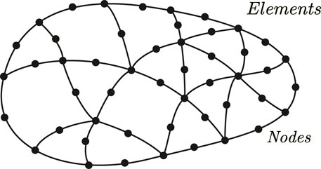
FIGURE 1. Elements of a 2D FEM model.

Galerkin Finite Element Method (GFEM)

In the Galerkin FEM, the weight function w in Eq. 6 is taken as the shape function $N_c$, i.e., $w=N_c$, with the subscript c representing the element nodal number corresponding to the collocation point c. Thus, for an element e with a domain ${\mathrm{\Omega }}_e$ bounded by the boundary ${\mathrm{\Gamma }}_e$, Eq. 6 results in the following element equation:

$\underset{K_{ec}}{\underbrace{{\int }_{{\mathrm{\Omega }}_e}\frac{\partial N_c}{\partial x_l}{D}_{ijkl}\frac{\partial N_{\alpha }}{\partial x_j}d\mathrm{\Omega }{u}_k^{\alpha }}}=\underset{F_{ec}^t}{\underbrace{{\int }_{{\mathrm{\Gamma }}_e}{N}_c{t}_i\left(\mathit{x}\right)d\mathrm{\Gamma }}}+\underset{F_{ec}^b}{\underbrace{{\int }_{{\mathrm{\Omega }}_e}{N}_c{b}_{i}d\mathrm{\Omega }}}(9)$

where the left-hand side is related to the so-called element stiffness term and the right-hand side is the total equivalent load of element e.

We assume that the problem is discretized as N computational points, and each point is shared by a number of elements. Thus, for a point n, assembling all related elements’ contributions from Eq. 9, it follows that

${\displaystyle \sum _{e_n{c}_n=1}^{E_n}}{K}_{e_n{c}_n}={\displaystyle \sum _{e_n{c}_n=1}^{E_n}}{F}_{e_n{c}_n}^t+{\displaystyle \sum _{e_n{c}_n=1}^{E_n}}{F}_{e_n{c}_n}^b(10)$

where $E_n$ is the number of elements connected to point n and $e_n{c}_n$ represents the element e connected to point n at the element node c, which corresponds to point n. It is noted that for one element among all element nodes, only one node corresponds to point n.

In Eq. 10, the equivalent traction load, the second term in Eq. 10, has different values for interface and out boundary points, i.e.,

$\begin{array}{l}{\displaystyle \sum _{e_n{c}_n=1}^{E_n}}{F}_{e_n{c}_n}^t=0,\mathrm{w}\mathrm{h}\mathrm{e}\mathrm{n}n\mathrm{i}\mathrm{s}\mathrm{a}\mathrm{t}\mathrm{i}\mathrm{n}\mathrm{t}\mathrm{e}\mathrm{r}\mathrm{f}\mathrm{a}\mathrm{c}\mathrm{e}\mathrm{n}\mathrm{o}\mathrm{d}\mathrm{e}\mathrm{s}\\ {\displaystyle \sum _{e_n{c}_n=1}^{E_n}}{F}_{e_n{c}_n}^t={\displaystyle \sum _{e_n{c}_n=1}^{E_n}}{\int }_{\mathrm{\Gamma }{e}_n}{N}_{c_n}{t}_{i}d\mathrm{\Gamma },\mathrm{w}\mathrm{h}\mathrm{e}\mathrm{n}n\mathrm{i}\mathrm{s}\mathrm{a}\mathrm{t}\mathrm{o}\mathrm{u}\mathrm{t}\mathrm{b}\mathrm{o}\mathrm{u}\mathrm{n}\mathrm{d}\mathrm{a}\mathrm{r}\mathrm{y}\mathrm{n}\mathrm{o}\mathrm{d}\mathrm{e}\mathrm{s}\end{array}(11)$

where ${\mathrm{\Gamma }}_{en}$ is the out boundary of element e including point n and $N_{c_n}$ is the shape function of the element node c corresponding to point n. The first equation in (11) comes from the fact that the equivalent traction loads from opposite surfaces of the related elements including the interface point are counteracted by one another, and the second equation in (11) relies on the characteristics of the shape function $N_{c_n}$, where its value is zero on the surfaces excluding node $c_n$.

When n in Eq. 10 goes through all the N points, the following system of equations can be produced in the matrix form:

$\mathit{K}\mathit{u}=\mathit{F}(12)$

where K is the global stiffness matrix, u the displacement vector, and F the total equivalent load vector.

The Galerkin FEM results in a symmetric and a banded sparse coefficient matrix K in the system of equations; this makes the method very efficient and stable. In particular, when some modern techniques are integrated into FEM, such as the control volume finite-element method [18, 19], isogemetric technique [20, 21], and gradient smoothing technique [22, 23], quite complicated engineering problems can be efficiently solved. Moreover, in recent years, a number of newly proposed FEMs have been developed, as described below.

Surface-Volume–Based Finite Element Method (SVFEM)

The Galerkin FEM presented above is derived based on the volume-based weighted residual formulation (6). In the article, another type of FEM can be generated based on the surface-volume–based weighted residual formulation (7), which has the same element discretisation as Figure 1. To do this, as done above, by applying Eq. 7 to an element domain, say element e, and by using $w=N_c$ and substituting Eq. 8 into Eq. 7, it follows that

$\underset{K_{ec}^{\mathrm{\Gamma }}}{\underbrace{{\int }_{{\mathrm{\Gamma }}_e}\frac{\partial N_c}{\partial x_l}{D}_{ijkl}{n}_j{N}_{\alpha }d\mathrm{\Gamma }{u}_k^{\alpha }}}-\underset{K_{ec}^{\mathrm{\Omega }}}{\underbrace{{\int }_{{\mathrm{\Omega }}_e}\frac{\partial }{\partial x_j}\left(D_{ijkl}\frac{\partial N_c}{\partial x_l}\right)N_{\alpha }d\mathrm{\Omega }{u}_k^{\alpha }}}=\underset{F_{ec}^t}{\underbrace{{\int }_{{\mathrm{\Gamma }}_e}{N}_c{t}_i\left(\mathit{x}\right)d\mathrm{\Gamma }}}+\underset{F_{ec}^b}{\underbrace{{\int }_{{\mathrm{\Omega }}_e}{N}_c{b}_{i}d\mathrm{\Omega }}}(13)$

Similar to Eq. 10, for the computational point n, assembling all related elements’ contributions from Eq. 13, the following equation can be formed:

${\displaystyle \sum _{e_n{c}_n=1}^{E_n}}{K}_{e_n{c}_n}^{\mathrm{\Gamma }}-{\displaystyle \sum _{e_n{c}_n=1}^{E_n}}{K}_{e_n{c}_n}^{\mathrm{\Omega }}={\displaystyle \sum _{e_n{c}_n=1}^{E_n}}{F}_{e_n{c}_n}^t+{\displaystyle \sum _{e_n{c}_n=1}^{E_n}}{F}_{e_n{c}_n}^b(14)$

The right-hand side of Eq. 14 is exactly the same as that of the standard Galerkin FEM, as shown in Eq. 11.

When n in Eq. 14 goes through all the N discretized points, the following system of equations can be produced in the matrix form:

$\stackrel{\sim }{\mathit{K}}\mathit{u}=\mathit{F}(15)$

In the above equation, $\stackrel{\sim }{\mathit{K}}$ is also called as the global stiffness matrix and is band-sparse, but it is not symmetric anymore; u and F are the same as in Eq. 12.

Although $\stackrel{\sim }{\mathit{K}}$ in SVFEM is not symmetric and this could reduce the solution efficiency to a certain level, Eq. 15 would give more accurate results than Eq. 12 since more mathematical treatments have been performed in Eq. 13 than in Eq. 9.

The SVFEM presented above is included in the new research work by the article’s authors. Some results have not yet been published in the literature; however, and they will be put in the public domain in the near future.

Strong-Form Volume-Operation–Based Methods

The above-described Galerkin FEM and SVFEM are weak-form algorithms, which require integration over elements to form the system of equations. In recent years, new types of strong-form FEM-like volume-operation–based methods have been proposed, which belong to a type of element collocation method and do not need integration computations. However, the stability of the strong-form algorithms is usually not as good as the weak-form algorithms, although for general problems these algorithms can still give satisfactory results.

Wen and Li et al. [8, 24] proposed the finite block method (FBM) in 2014, in which isoparametric element-like blocks are used to compute the first-order partial derivative of physical variables with respect to the global coordinates. FBM has the advantage of simple coding, and since element-like blocks are used, the stability of the solution is usually good. On the other hand, since all nodal values of physical variables over each block are independently inserted into the system of equations by introducing a consistent condition of physical variables and an equilibrium condition of the physical variable gradient in the system, there are more unknowns in the formed final system of equations than other frequently used numerical methods in the case of the same number of total nodes. In view of this issue, as few blocks as possible should be used when solving a problem using FBM to ensure that the final system of equations is not so large.

In the same period, Fantuzzi et al. [25, 26] proposed another type of strong-form FEM (SFEM), in which a set of formulations computing the first- and second-order spatial partial derivatives are derived for 2D problems and are used to collocate the governing PDEs in solid mechanics. In SFEM, the continuity condition among elements is determined by the compatibility, and a mapping technique is used to transform both the governing differential equations and the compatibility conditions between two adjacent sub-domains into the regular master element in the computational space. As in FBM, the treatment of the compatibility and equilibrium conditions between elements is still complicated; this makes SFEM not as flexible as GFEM when solving complicated engineering problems.

In 2017, Gao et al. [27] proposed a new type of strong-form FEM, called the Element Differential Method (EDM), for solving heat conduction problems, and later it was successfully used to solve solid mechanics [4, 28], electromagnetic [29], and thermo-mechanical-seepage coupled [30] problems. As in FBM, Lagrange polynomials are used to construct high-order elements in EDM. The essential difference between EDM and FBM is that both the first- and second-order partial derivatives were derived for 2D and 3D problems in EDM. The following is a brief review of EDM.

Looking back at Eq. 8 for physical variable interpolation over an element, the global coordinates can also be expressed by their nodal values and shape functions, as follows:

$x_i=N_{\alpha }{x}_i^{\alpha }(16)$

Based on Eqs 8, 16, the following expressions can be derived for the first- and second-order partial derivatives [4, 27]:

$\frac{\partial u_k}{\partial x_i}=d_i^{c{\alpha }^{\prime }}{u}_k^{{\alpha }^{\prime }}(17)$

$\frac{{\partial }^2{u}_k}{\partial x_i\partial x_j}=d_{ij}^{c{\alpha }^{″}}{u}_k^{{\alpha }^{″}}(18)$

where

$d_i^{c{\alpha }^{\prime }}=\frac{\partial N_{\alpha }}{\partial x_i}={\left[J\right]}_{ik}^{-1}\frac{\partial N_{\alpha }}{\partial {\xi }_k}(\mathrm{19a})$

$d_{ij}^{c{\alpha }^{″}}=\frac{{\partial }^2{N}_{\alpha }}{\partial x_i\partial x_j}=\left[{\left[J\right]}_{ik}^{-1}\frac{{\partial }^2{N}_{\alpha }}{\partial {\xi }_k\partial {\xi }_l}+\frac{\partial {\left[J\right]}_{ik}^{-1}}{\partial {\xi }_l}\frac{\partial N_{\alpha }}{\partial {\xi }_k}\right]\frac{\partial {\xi }_l}{\partial x_j}(\mathrm{19b})$

where $\left[J\right]=\left[\partial \mathit{x}/\partial \mathit{\xi }\right]$ is the Jacobian matrix between the global coordinate x and the local coordinate $\mathit{\xi }$ of the element. The detailed expressions for each term in Eqs 19a, 19b can be found in [27, 28].

The main advantage of the strong-form FEMs over weak-form FEMs is that the derived spatial partial derivatives can be directly substituted into the problem’s PEDs and B.C. to set up the system of equations. For example, by using Eqs 17, 18, the PDE and B.C. for the solid mechanics shown in Eqs 3, 4 can be directly used to generate the following discretized equations:

$d_l^{c{\beta }^{\prime }}{D}_{ijkl}\left({\mathit{x}}^{{\beta }^{\prime }}\right)d_j^{{\beta }^{\prime }{\alpha }^{\prime }}{u}_k^{{\alpha }^{\prime }}+b_i\left({\mathit{x}}^c\right)=0,{\mathit{x}}^c\in {\mathrm{\Omega }}_e(20)$

$\left\{\begin{array}{l}{u}_i\left({\mathit{x}}^c\right)={\overline{u}}_i,{\mathit{x}}^c\in {\mathrm{\Gamma }}_u\\ D_{ijkl}\left({\mathit{x}}^c\right)n_j\left({\mathit{x}}^c\right)d_l^{c{\alpha }^{\prime }}{u}_k^{{\alpha }^{\prime }}={\overline{t}}_i\left({\mathit{x}}^c\right),{\mathit{x}}^c\in {\mathrm{\Gamma }}_t\end{array}\right.(21)$

In the above equations, ${\mathrm{\Gamma }}_u$ and ${\mathrm{\Gamma }}_t$ are the out boundaries of the problem, over which the displacement and traction boundary conditions are specified. The big issue in the strong-form FEM is how to set up the discretized equation when the collocation point ${\mathit{x}}^c$ is located on the interface ${\mathrm{\Gamma }}_I$ between elements. To solve this issue, Gao et al. [4, 27] proposed the summation-equilibrium technique for all related tractions, that is, ${\displaystyle \sum }_{e=1,s=1}{t}_i^{es}=0$, to form a single set of equations at an element interface node, which can be expressed as

${\displaystyle \sum _{e=1,s=1}^{E_c}}{D}_{ijkl}^e\left({\mathit{x}}^c\right)n_j^{es}\left({\mathit{x}}^c\right)d_l^{ec{\alpha }^{\prime }}{u}_k^{e{\alpha }^{\prime }}=0,{\mathit{x}}^c\in {\mathrm{\Gamma }}_I(22)$

where $E_c$ is the number of all elements connected with the interface collocation point c. Various numerical examples [27–31] have proved that the above equation can give correct results. The important point is that Eq. 22 allows the final system of equations to have the same size as the conventional FEM, which is much smaller than those in FBM [8] and SFEM [25].

Surface-Operation–Based Methods

Surface-operation–based numerical methods include the finite volume method (FVM), boundary element method (BEM), etc., which are operated mainly on the surfaces of a control volume or on the boundary of the considered problem.

Finite Volume Method (FVM)

The FVM looks like a volume-based method [32–35]. However, in this article, it is classified into the category of surface-operation–based methods. This is because its main operation is over the surfaces of the control volume, rather than on the volume itself. To see this, let us take the weight function w to be 1 in Eq. 6. This results in the following:

${\int }_{\mathrm{\Gamma }}{t}_{i}d\mathrm{\Gamma }+{\int }_{\mathrm{\Omega }}{b}_{i}d\mathrm{\Omega }=0(23)$

In FVM, the computational domain is discretized into a series of control volumes [32]. Applying Eq. 23 to each control volume, say volume ${\mathrm{\Omega }}_c$, and dividing its boundary $\partial {\mathrm{\Omega }}_c$ into two parts, the inner boundary ${\mathrm{\Gamma }}_{Ic}$ and outer boundary ${\mathrm{\Gamma }}_{oc}$, Eq. 23 can be written as:

${\int }_{{\mathrm{\Gamma }}_{Ic}}{D}_{ijkl}{n}_j\frac{\partial u_k}{\partial x_l}d\mathrm{\Gamma }+{\int }_{{\mathrm{\Gamma }}_{oc}}{\overline{t}}_{i}d\mathrm{\Gamma }+{\int }_{{\mathrm{\Omega }}_c}{b}_{i}d\mathrm{\Omega }=0(24)$

where ${\mathrm{\Gamma }}_{Ic}\cup {\mathrm{\Gamma }}_{oc}=\partial {\mathrm{\Omega }}_c$.

Equation 24 is a typical formulation of FVM, from which we can see that the main computation is over the control surfaces of a control volume. The key work in FVM is the evaluation of the physical variable gradient $\partial u_k/\partial x_l$ included in the first control surface integral of Eq. 24 [36, 37]. In the conventional FVM, the interface ${\mathrm{\Gamma }}_{Ic}$ is taken as the mid-surface connected by the collocation point c and around-neighbour points; thus, $\partial u_k/\partial x_l$ at the mid-surface can be easily computed using the values of $u_k$ between c and the neighbour points [38–40]. However, only the linear variation of $u_k$ over the operation surface can be easily achieved. It is difficult to construct a high-order scheme to compute the value of $\partial u_k/\partial x_l$ on the operation surface. To overcome this problem, the free element [15, 31] can be used in FVM analysis.

Free Element-Based FVM (FEFVM)

In [15], the free element method (FrEM) was proposed for thermal-mechanical analysis. In FrEM, the isoparametric elements used in FEM are defined at each collocation point, as shown in Figure 2. The weak-form formulation of FrEM has the form shown in Eq. 24 [31]; however, the control volume is taken as the free element, as shown in Figure 2. Generally, for a free element, some of its operation surfaces are located inside the domain and some on the outer boundary of the problem, as shown in Figure 2. For this case, both the inner surface integral over ${\mathrm{\Gamma }}_{Ic}$ and outer surface integral over ${\mathrm{\Gamma }}_{oc}$ will appear in Eq. 24.

FIGURE 2

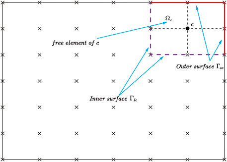
FIGURE 2. Operation surfaces ${\mathrm{\Gamma }}_{Ic}$ and ${\mathrm{\Gamma }}_{oc}$ formed by the boundary of the free element built for collocation point c.

However, when all the surfaces of the free element formed for the collocation c are located within the problem, as shown in Figure 3, only the inner surface integral exists.

FIGURE 3

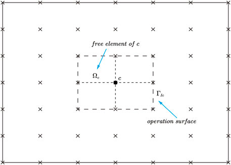
FIGURE 3. Operation surface ${\mathrm{\Gamma }}_{Ic}$ of the free element completely included in the computational domain.

In this case, Eq. 24 takes the following form:

${\int }_{{\mathrm{\Gamma }}_{Ic}}{D}_{ijkl}{n}_j\frac{\partial u_k}{\partial x_l}d\mathrm{\Gamma }+{\int }_{{\mathrm{\Omega }}_c}{b}_{i}d\mathrm{\Omega }=0(25)$

Since high-order free elements can be easily formed in FrEM [15], a high accuracy of $\partial u_k/\partial x_l$ in FEFVM can be easily achieved. A set of analytical expressions for computing $\partial u_k/\partial x_l$ over a free element have been derived in [4]. Although it is easy to set up a high-order free element, the accuracy of $\partial u_k/\partial x_l$ is not high. This is because its value is taken on the boundary of ${\mathrm{\Omega }}_c$, which is not as accurate as inside a free element. To overcome this drawback, the element-shell–strengthened FVM is proposed in the following section.

Element-Shell Enhanced FVM (ESFVM)

To improve the accuracy of $\partial u_k/\partial x_l$ included in the first boundary integral of Eq. 24, additional free elements are formed for each side/surface of the collocation element ${\mathrm{\Omega }}_c$, which form an element ring/shell for 2D/3D control sides/surfaces, as shown in Figure 4 for a 2D case.

FIGURE 4

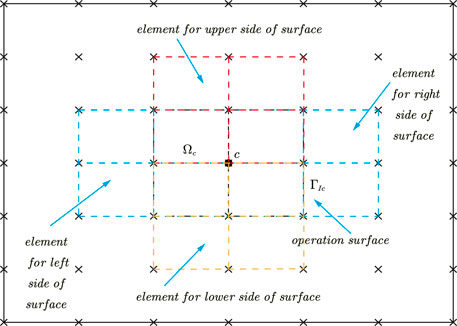
FIGURE 4. Free elements around the operation surfaces.

In this strategy, the inner surface integral included in Eq. 24 can be written as follows:

${\int }_{{\mathrm{\Gamma }}_{Ic}}{D}_{ijkl}{n}_j\frac{\partial u_k}{\partial x_l}d\mathrm{\Gamma }={\displaystyle \sum _{s=1}^{N_{Is}}}{\int }_{{\mathrm{\Gamma }}_s}{D}_{ijkl}{n}_j\frac{\partial u_k}{\partial x_l}\left(x^s\right)d\mathrm{\Gamma }\left(x^s\right)(26)$

where $N_{Is}$ is the number of inner operation surfaces of the control volume ${\mathrm{\Omega }}_c$, which is 4 in the case shown in Figure 4 and $x^s$ denotes the coordinate of the integration point over a surface s. In ESFVM, the first spatial derivative term included in the right-hand side of Eq. 26 is evaluated by the free element of the element-shell including the operation surface under integration, and thus, using Eq. 17 it follows that

${\int }_{{\mathrm{\Gamma }}_s}{D}_{ijkl}{n}_j\frac{\partial u_k}{\partial x_l}\left(x^s\right)d\mathrm{\Gamma }\left(x^s\right)={\int }_{{\mathrm{\Gamma }}_s}{D}_{ijkl}{n}_j{d}_i^{s{\alpha }^{\prime }}\left(x^s\right)d\mathrm{\Gamma }\left(x^s\right)u_k^{{\alpha }^{\prime }}(27)$

where $d_i^{s{\alpha }^{\prime }}$ is computed using the free element formed for the surface s.

In ESFVM, since the operation surfaces of ${\mathrm{\Omega }}_c$ are included in the additional formed elements, the accuracy of $\partial u_k/\partial x_l$ is higher than using the same element ${\mathrm{\Omega }}_c$ built for point c.

Evaluation of the Domain Integral Involved in FVM

When the body force is considered in the computational problem, the FVM equations inevitably involve the domain integrals, as shown in Eqs 23–25. Evaluation of the involved domain integrals is troublesome work. In conventional FVM, for achieving high efficiency, the domain integral is evaluated by assuming that the body force is constant throughout the control volume [41]. Thus, the domain integral can be simply written as

${\int }_{{\mathrm{\Omega }}_c}{b}_{i}d\mathrm{\Omega }={\overline{b}}_i{\mathrm{\Omega }}_c(28)$

where ${\overline{b}}_i$ is the average value of $b_i$ in the control volume ${\mathrm{\Omega }}_c$.

Obviously, if $b_i$ is sharply changeable in ${\mathrm{\Omega }}_c$, the above evaluation gives rise to a large error. To overcome this issue and for a universal scheme to accurately evaluate the domain integral, the Radial Integration Method (RIM) [42] can be employed to evaluate the domain integral in Eq. 28, which can be expressed as

${\int }_{{\mathrm{\Omega }}_c}{b}_{i}d\mathrm{\Omega }={\int }_{\partial {\mathrm{\Omega }}_c}\frac{F_i}{r^n\left(c,\mathrm{\Gamma }\right)}\frac{\partial r}{\partial n}d\mathrm{\Gamma }(29)$

where $\partial {\mathrm{\Omega }}_c$ is the boundary of the control volume ${\mathrm{\Omega }}_c$, $r\left(c,\mathrm{\Gamma }\right)$ is the distance from the collocation point c to the boundary $\mathrm{\Gamma }$, n is 1 or 2 for 2D or 3D problem, and

$F_i={\int }_0^{r\left(\mathrm{c},\mathrm{\Gamma }\right)}{b}_i{r}^{n}dr(30)$

For most cases, $b_i$ is a known function and Eq. 30 can be analytically integrated. For very complicated $b_i$, Eq. 30 can be evaluated using Gauss quadrature [42].

The above equations are suitable for any shaped control volume, regular or irregular, since the integration is over the boundary of ${\mathrm{\Omega }}_c$. In FEFVM and ESFVM, ${\mathrm{\Omega }}_c$ is the free element domain formed for the collocation point c and $\partial {\mathrm{\Omega }}_c$ is the boundary of the free element. Apart from the high accuracy, the main advantage of using RIM to evaluate the domain integral is that only the operation surfaces of the control volume are needed to evaluate the domain integral, with no need to perform volume integration over ${\mathrm{\Omega }}_c$.

Boundary Element Method (BEM)

In Eq. 7, if the weight function w is taken as the displacement fundamental solution $u_{mi}^{*}$ [9, 10], i.e., $w=u_{mi}^{*}$, the following BEM integral equation can be established:

${\int }_{\mathrm{\Gamma }}\frac{\partial u_{mi}^{*}}{\partial x_l}{D}_{ijkl}{n}_j{u}_{k}d\mathrm{\Gamma }-{\int }_{\mathrm{\Omega }}\frac{\partial }{\partial x_j}\left(D_{ijkl}\frac{\partial u_{mi}^{*}}{\partial x_l}\right)u_{k}d\mathrm{\Omega }={\int }_{\mathrm{\Gamma }}{u}_{mi}^{*}{t}_{i}d\mathrm{\Gamma }+{\int }_{\mathrm{\Omega }}{u}_{mi}^{*}{b}_{i}d\mathrm{\Omega }(31)$

Recalling that the displacement fundamental solution $u_{mi}^{*}$ satisfies the following equation:

$\frac{\partial }{\partial x_j}\left(D_{ijkl}\frac{\partial u_{mi}^{*}}{\partial x_l}\right)+{\delta }_{mk}\delta \left(p,q\right)=0(32)$

Equation 31 becomes

$u_m+{\int }_{\mathrm{\Gamma }}{t}_{mk}^{*}{u}_{k}d\mathrm{\Gamma }={\int }_{\mathrm{\Gamma }}{u}_{mi}^{*}{t}_{i}d\mathrm{\Gamma }+{\int }_{\mathrm{\Omega }}{u}_{mi}^{*}{b}_{i}d\mathrm{\Omega }(33)$

where

$t_{mk}^{*}=D_{ijkl}{n}_j\frac{\partial u_{mi}^{*}}{\partial x_l}(34)$

To evaluate the domain integral appearing in Eq. 33, the conventional technique is to discretize the domain into internal cells [9]; however, this eliminates the advantage of BEM where only the boundary of the problem needs to be discretized into elements. To overcome this drawback, a transformation technique is usually employed to transform the domain integral into an equivalent integral. The most extensively used transformation technique is the Dual Reciprocity Method [DRM] [43]. Another technique used is the Radial Integration Method (RIM) [42], which can give more accurate results than DRM.

Using RIM, the domain integral in Eq. 33 can be expressed as

${\int }_{\mathrm{\Omega }}{u}_{mi}^{*}{b}_{i}d\mathrm{\Omega }={\int }_{\mathrm{\Gamma }}\frac{F_{mi}}{r^n\left(p,q\right)}\frac{\partial r}{\partial n}d\mathrm{\Gamma }\left(q\right)(35)$

where the radial integral is

$F_{mi}={\int }_0^{r\left(p,q\right)}{u}_{mi}^{*}{b}_i{r}^{n}dr(36)$

where n = 1 for 2D problems and n = 2 for 3D problems. When $b_i$ is a known function, Eqs 35, 36 can give rise to a very accurate result. On the other hand, for the case where $b_i$ is not very complicated, Eq. 36 can be analytically integrated [42]. However, when $b_i$ is a complicated function, numerical integration should be performed [44].

Line-Operation–Based Methods

Line-operation–based methods include the conventional finite difference method (FDM) [12] and the recently proposed finite line method (FLM) [3, 13]. In these methods, the computational domain is discretized into a series of points and lines formed by around points are then used to compute the spatial partial derivatives included in the PDEs, as shown in Figure 5 for a 2D case. FDM constructs the first- and second-order partial derivatives using a line of points along the derivative directions. The main drawback of FDM is that if the lines that define the derivative directions are not orthogonal to one another in 2D or 3D problems, the accuracy of the cross-partial derivatives of different directions is usually very poor [45, 46]. This is why FDM cannot simulate irregular geometry problems well. In contrast, FLM has a much better performance in overcoming this drawback.

FIGURE 5

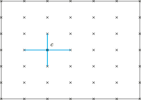
FIGURE 5. Line-set consisting of two crossed lines for a 2D problem.

FLM uses a number of lines, named a line-set, to set up the solution scheme. Usually, at a collocation point, two lines (for 2D problems) or three lines (for 3D problems) are used to form the line-set, as shown in Figure 5. Figure 6 shows the high-order line-sets of an internal collocation point for 2D and 3D problems.

FIGURE 6

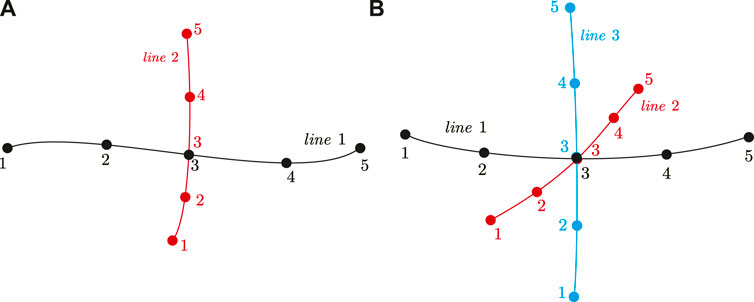
FIGURE 6. Node distributions over line-sets defined at 2D or 3D internal points. (A) 2D problem (B) 3D problem.

Along a line of a line-set, the coordinates and physical variables can be expressed as

$x_i={\displaystyle \sum _{\alpha =1}^m}{L}^{\alpha }\left(l\right)x_i^{\alpha }\equiv L^{\alpha }\left(l\right)x_i^{\alpha }(37)$

$u_k={\displaystyle \sum _{\alpha =1}^m}{L}^{\alpha }\left(l\right)u_k^{\alpha }\equiv L^{\alpha }\left(l\right)u_k^{\alpha }(38)$

where m is the number of nodes defined along a line of the line-set, l is the arclength measured from node 1, and $L^{\alpha }$ is the Lagrange polynomial:

$L^{\alpha }\left(l\right)={\displaystyle \prod _{\beta =1,\beta \ne \alpha }^m}\frac{l-l^{\beta }}{l^{\alpha }-l^{\beta }},\left(\alpha =1\sim m\right)(39)$

By differentiating Eqs 37, 38 with respect to l, we can obtain expressions for computing the first- and second-order partial derivatives at the collocation point ${\mathit{x}}^c$, as follows [3, 13]:

$\frac{\partial u_k\left({\mathit{x}}^c\right)}{\partial x_i}=d_i^{c{\alpha }^{\prime }}{u}_k^{{\alpha }^{\prime }}(40)$

$\frac{{\partial }^2{u}_k\left({\mathit{x}}^c\right)}{\partial x_i\partial x_j}=d_{ij}^{c{\alpha }^{″}}{u}_k^{{\alpha }^{″}}(41)$

where

$d_i^{c{\alpha }^{\prime }}={\left.{\displaystyle \sum _{I=1}^d}{\left[J\right]}_{iI}^{-1}\frac{\partial L_I^{\alpha }\left(l\right)}{\partial l}\right|}_{l=l\left({\mathit{x}}^c\right)}(42)$

$d_{ij}^{c{\alpha }^{″}}=d_j^{c{\beta }^{\prime }}{d}_i^{{\beta }^{\prime }{\alpha }^{\prime }}(43)$

where the repeated indexes represent summation, and d = 2 for 2D problems, d = 3 for 3D problems, and I represents the line number.

Using Eqs 40, 41, we can easily discretize a PDE and the related boundary conditions. For example, the PDE for the solid mechanics shown in Eqs 3, 4 can directly generate a set of discretized equations which have the same forms as those shown in Eqs 20, 21.

Point-Operation–Based Methods

Point-operation–based methods cover a number of numerical methods, such as the mesh free method (MFM) [5, 47–50], fundamental solution method [16], radial basis function method [51–53], and the newly developed free element method (FrEM) [15, 31]. In these types of methods, the computational domain is discretized into a series of points and solution schemes are established by collocating the governing PDEs or their integral forms at each collocation point. In MFM, the partial derivatives at the collocation point c are derived based on a group of scatter points within a specified support region around c, as shown in Figure 7A, while in FrEM, partial derivatives are derived based on an isoparametric element freely formed for point c, as shown in Figure 7B. In MFM and FrEM, both weak-form and strong-form solution schemes are available. In the following sections, the two schemes of FrEM will be described in detail.

FIGURE 7

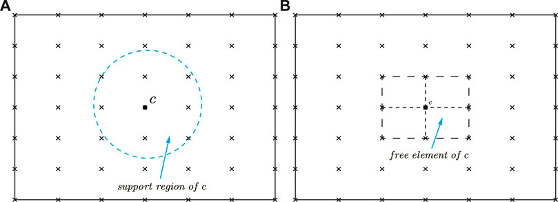
FIGURE 7. 2D patterns for MFM (A) and FrEM (B) at a collocation point.

Weak-Form Free Element Method (WFrEM)

In FrEM, a free element is independently formed for each collocation point c [31], with the domain denoted by ${\mathrm{\Omega }}_c$. The shape function shown in Eq. 8 is still employed for the formed free element. Let us apply the weighted residual formulation (6) to ${\mathrm{\Omega }}_c$ and take the weight function as the shape function of the collocation point c, i.e., $w=N_c$. Thus, the following equation can be obtained:

${\int }_{{\mathrm{\Omega }}_c}\frac{\partial N_c}{\partial x_l}{D}_{ijkl}\frac{\partial u_k}{\partial x_j}d\mathrm{\Omega }={\int }_{\partial {\mathrm{\Omega }}_c}{N}_c{t}_i\left(\mathit{x}\right)d\mathrm{\Gamma }+{\int }_{{\mathrm{\Omega }}_c}{N}_c{b}_{i}d\mathrm{\Omega }(44)$

where the derivatives of the shape functions are computed using Eq. 19a.

Dividing the boundary $\partial {\mathrm{\Omega }}_c$ of ${\mathrm{\Omega }}_c$ into two parts; the inner boundary ${\mathrm{\Gamma }}_{Ic}$, which is located within the problem and the outer boundary ${\mathrm{\Gamma }}_{oc}$, which is located on the outer surface of the problem. Remembering that $N_c$ is zero on the surfaces excluding point c, making the integral over ${\mathrm{\Gamma }}_{Ic}$ zero, as a result, Eq. 44 can be written as:

${\int }_{{\mathrm{\Omega }}_c}\frac{\partial N_c}{\partial x_l}{D}_{ijkl}\frac{\partial N_{\alpha }}{\partial x_j}d\mathrm{\Omega }{u}_k^{\alpha }={\int }_{{\mathrm{\Gamma }}_{oc}}{N}_c{\overline{t}}_{i}d\mathrm{\Gamma }+{\int }_{{\mathrm{\Omega }}_c}{N}_c{b}_{i}d\mathrm{\Omega }(45)$

where ${\mathrm{\Gamma }}_{oc}=\partial {\mathrm{\Omega }}_c\cap \partial \mathrm{\Omega }$, which is the outer boundary containing c.

From Eq. 45, it can be seen that the form of the basic equation in WFrEM is similar to that in the conventional FEM. The essential difference between them is that the element in WFrEM is freely formed at each collocation point, the nodes of which are not restricted to any particular nodes of adjacent elements. It is also noteworthy that the free elements formed by around-collocation points are overlapped in FrEM since they are formed locally and independently at each point.

Strong-Form Free Element Method (SFrEM)

The SFrEM is a type of collocation method [15]. To achieve a highly accurate result, the collocation point c should be placed inside the formed free element. For this reason, the free elements used should have at least one internal node. In principle, any type of isoparametric elements with internal nodes can be utilized in SFrEM analysis [54–56]. For example, Figure 8 shows new types of quadratic triangular and tetrahedral elements [55] and Figure 9 shows a 21-noded block element [15].

FIGURE 8

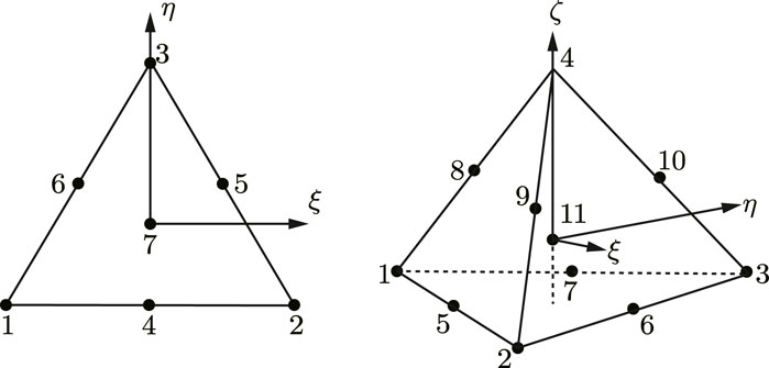
FIGURE 8. Quadratic 7-noded triangular and 11-noded tetrahedral elements.

FIGURE 9

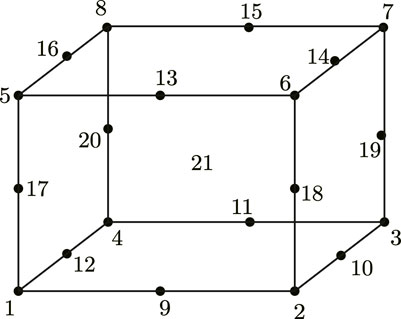
FIGURE 9. 21-noded 3D quadratic block element.

The shape functions for the above triangular and tetrahedral elements can be found in [55] and that for the 21-noded quadratic block element in [15].

For higher-order elements, the best method is to use Lagrange elements. For example, Figure 10 shows a 16-noded 2D third-order Lagrange element.

FIGURE 10

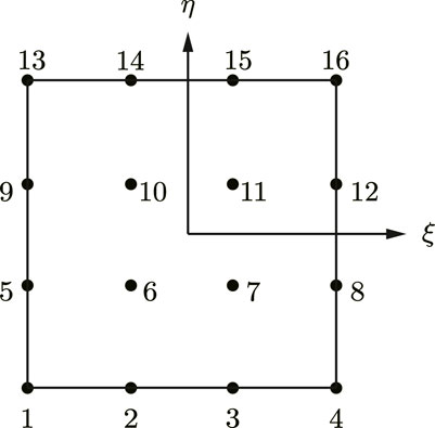
FIGURE 10. 16-noded 2D third-order Lagrange element.

The shape functions of Lagrange elements for 2D and 3D problems can be constructed as follows [4]:

$\begin{array}{l}{N}_{\alpha }\left(\xi ,\eta \right)=L^I\left(\xi \right)L^J\left(\eta \right),for2D\\ N_{\alpha }\left(\xi ,\eta ,\zeta \right)=L^I\left(\xi \right)L^J\left(\eta \right)L^K\left(\zeta \right),for3D\end{array}(46)$

where $L^I,L^J,\mathrm{a}\mathrm{n}\mathrm{d}{L}^K$ are determined by Eq. 39 and the superscript α is determined by the permutation of subscripts I, J, and K sequentially.

From the shape functions shown in Eq. 46, the analytical expressions for computing the first- and second-order partial derivatives can be derived, which are the same as those shown in Eqs 17–19a, 19b. The collocation scheme to form the system of equations for the governing PDEs is the same as that in EDM, shown in Eqs 20, 21, the difference being that in SFrEM, only the interior and out boundary nodes are used.

Numerical Examples

To demonstrate the performances of some of the numerical methods described in the article, a dual-struts supersonic combustor [57] is simulated in the following. The physical problem and relevant dimensions are shown in Figure 11. The Yong’s modulus and Poison ratio of all materials in the problem are taken as $E=206GPa$ and $\nu =0.3$. To constrain the four frames supporting the combustor, the lower surface of the left frame is fixed and the lower surfaces of the other three frames are free only in the longitudinal direction (x-direction). All remaining outer surfaces of the combustor are imposed with a traction-free boundary condition. Pressure loads are applied on the inner surfaces of the combustor, which are distributed along the x-direction, as shown in Figure 12.

FIGURE 11

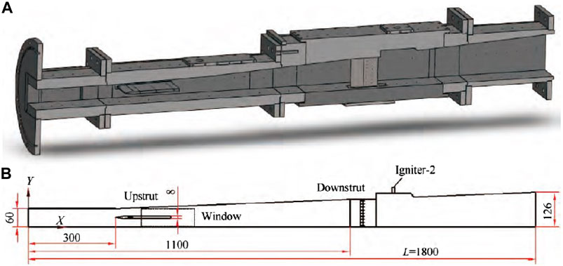
FIGURE 11. Configurations of a combustion chamber with tow struts.

FIGURE 12

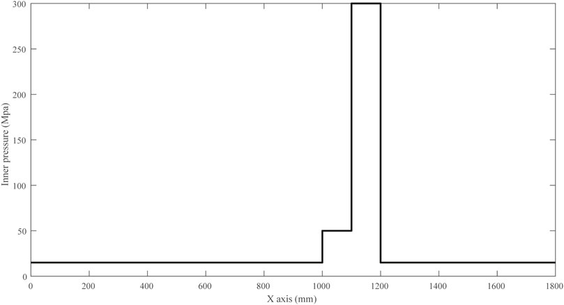
FIGURE 12. Pressure applied on the inner surfaces of the combustor.

To simulate the problem using some of the described methods above, the whole structure is discretized into different numbers of nodes. Figure 13 shows the computational mesh connected by all finite lines in the FLM model with 657,582 nodes. Figure 14 shows a contour plot of the computed displacement amplitude over the deformed FLM mesh, with displacements enhanced ×20. For comparison, the problem is also computed using the FEM software ABAQUS, employing the same level nodes as those used in FLM. Figure 15 shows the comparison of the computed displacement amplitude along the line MN using four different methods; ABAQUS (FEM), finite line method (FLM), weak-form free element method (WFrEM), and the strong-form method (SFrEM). For the last two methods, two meshes with different numbers of nodes are used, in which WFrEM-880k indicates the result of WFrEM using 880,000 nodes. To clearly examine the differences between the different methods, Figure 16 shows the enhanced curves along two local parts of the line MN.

FIGURE 13

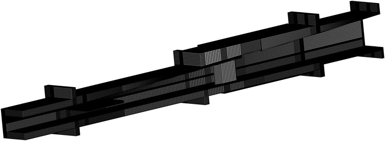
FIGURE 13. Computational mesh used in FLM analysis.

FIGURE 14

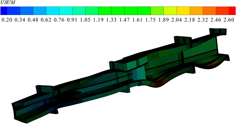
FIGURE 14. Contours of the deformed mesh, with displacements multiplied ×20.

FIGURE 15

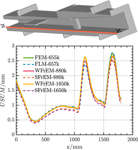
FIGURE 15. Computed displacements along the line MN using the four different methods.

FIGURE 16

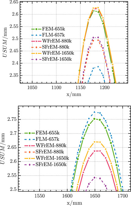
FIGURE 16. Enhanced curves along two parts of line MN.

From Figure 14, it can be seen that the deformations of two areas after the struts are large. This is because the combustion occurs immediately after the two struts; thus, the temperature and pressure are higher in these areas than other areas. Moreover, from Figure 15, it can be seen that all the computed results are in good agreement globally; this indicates that the methods presented in the article can handle real, complicated engineering problems. On the other hand, from Figure 16, it can be observed that the weak-form free element method (WFrEM) and the finite line method (FLM) give results closer to the finite element method (FEM). The essential reasons for this are that in WFrEM, numerical integration is performed over each free element, which is similar to FEM, giving very stable and accurate results. In FLM, the recursive technique is employed to evaluate the high-order derivatives, as shown in Eq. 43, making more points contribute to each collocation point [3]; therefore, more stable and accurate results can be obtained using FLM over other strong-form solution schemes [50].

Summary

In this article, four types of numerical methods are overviewed, most of which are newly proposed methods in recent years. Classification of all numerical methods into volume, surface, line, and point operation methods is performed for the first time in this article. This classification is conceptually clear and helpful for readers to understand the discretisation of problems and to realize the advantages and disadvantages of the different methods. Computational experience shows that the finite element, weak-form free element, and finite line methods have excellent performances.

Author Contributions

X-WG: conceptualization; investigation; methodology; software; project administration; resources; writing- original draft; supervision. W-WJ: software; validation; writing—review and editing; X-BX, H-YL, KY, JL, and MC: writing—review and editing. All authors contributed to the article and approved the submitted version.

Funding

We gratefully acknowledge support of this investigation by the National Natural Science Foundation of China under Grant No. 12072064 and the Fundamental Research Funds for Central Universities under Grant No. DUT22YG204.

Conflict of Interest

The authors declare that the research was conducted in the absence of any commercial or financial relationships that could be construed as a potential conflict of interest.

References

1. Coleman, C. J., On the use of radial basis functions in the solution of elliptic boundary value problems. Comput Mech (1996) 17:418–22. doi:10.1007/BF00363985

CrossRef Full Text | Google Scholar

2. Wang, Z. G., Liu, L. S., and Wu, Y. H., The unique solution of boundary value problems for nonlinear second-order integral-differential equations of mixed type in Banach spaces. Comput Math Appl (2007) 54:1293–301. doi:10.1016/j.camwa.2007.04.018

CrossRef Full Text | Google Scholar

3. Gao, X. W., Ding, J. X., and Liu, H. Y., Finite line method and its application in coupled heat transfer between fluid-solid domains. Acta Phys Sin (2022) 71(19):190201. doi:10.7498/aps.71.20220833

CrossRef Full Text | Google Scholar

4. Gao, XW, Li, ZY, Yang, K, Lv, J, Peng, HF, Cui, M, et al. Element differential method and its application in thermal-mechanical problems. Int J Numer Methods Eng (2018) 113(1):82–108. doi:10.1002/nme.5604

CrossRef Full Text | Google Scholar

5. Liu, GR. An overview on meshfree methods: For computational solid mechanics. Int J Comp Meth-sing (2016) 13(5):1630001. doi:10.1142/S0219876216300014

CrossRef Full Text | Google Scholar

6. Zienkiewicz, OC, Taylor, RL, and Fox, DD. The finite element method for solid and structural mechanics. Amsterdam: Elsevier (2014). p. 624.

Google Scholar

7. Hughes, TJR. The finite element method: Linear static and dynamic finite element analysis. Englewood Cliffs, NJ, USA: Prentice-Hall (1987). 704.

Google Scholar

8. Wen, PH, Cao, P, and Korakianitis, T. Finite block method in elasticity. Eng Anal Bound Elem (2014) 46:116–25. doi:10.1016/j.enganabound.2014.05.006

CrossRef Full Text | Google Scholar

9. Brebbia, CA, and Dominguez, J. Boundary elements: An introductory course. London, UK: McGraw-Hill Book Co (1992). 860.

Google Scholar

10. Gao, XW, and Davies, TG. Boundary element programming in mechanics. Cambridge, UK: Cambridge University Press (2002). 253.

Google Scholar

11. Onate, E, Cervera, M, and Zienkiewicz, OC. A finite volume format for structural mechanics. Int J Numer Meth Eng (1994) 37(2):181–201. doi:10.1002/nme.1620370202

CrossRef Full Text | Google Scholar

12. Wang, H, Dai, W, Nassar, R, and Melnik, R. A finite difference method for studying thermal deformation in a thin film exposed to ultrashort-pulsed lasers. Int J Heat Mass Tran (2006) 51:2712–23. doi:10.1016/j.ijheatmasstransfer.2006.01.013

CrossRef Full Text | Google Scholar

13. Gao, XW, Zhu, YM, and Pan, T. Finite line method for solving high-order partial differential equations in science and engineering. Part Diff Eq Appl Math (2023) 7:100477. doi:10.1016/j.padiff.2022.100477

CrossRef Full Text | Google Scholar

14. Atluri, SN, and Shen, SP. The meshless local Petrov-Galerkin (MLPG) method. Henderson, NV, USA: Tech Sci (2002). 51.

Google Scholar

15. Gao, XW, Gao, LF, Zhang, Y, Cui, M, and Lv, J. Free element collocation method: A new method combining advantages of finite element and mesh free methods. Comput Struct (2019) 215:10–26. doi:10.1016/j.compstruc.2019.02.002

CrossRef Full Text | Google Scholar

16. Fan, CM, Huang, YK, Chen, CS, and Kuo, SR. Localized method of fundamental solutions for solving two-dimensional Laplace and biharmonic equations. Eng Anal Bound Elem (2019) 101:188–97. doi:10.1016/j.enganabound.2018.11.008

CrossRef Full Text | Google Scholar

17. Belytschko, T, Liu, WK, Moran, B, and Elkhodary, K. Nonlinear finite elements for continua and structures. New York, USA: John Wiley and Sons (2000). 650.

Google Scholar

18. Baliga, BR. A control-volume based finite element method for convective heat and mass transfer. [PhD’s thesis]. Minnesota: University of Minnesota (1978).

19. Schneider, GE, and Raw, MJ. Control volume finite-element method for heat transfer and fluid-flow using colocated Variables.1.Computational procedure. Numer Heat Tr (1987) 11(4):363–90. doi:10.1080/10407798708552552

CrossRef Full Text | Google Scholar

20. Hughes, TJR, Cottrell, JA, and Bazilevs, Y. Isogeometric analysis: CAD, finite elements, NURBS,exact geometry and mesh refinement. Comput Methods Appl Mech Eng (2005) 194:4135–95. doi:10.1016/j.cma.2004.10.008

CrossRef Full Text | Google Scholar

21. Hou, WB, Jiang, K, Zhu, XF, Shen, Y., Li, Y, Zhang, X, et al. Extended Isogeometric Analysis with strong imposing essential boundary conditions for weak discontinuous problems using B++ splines. Comput Method Appl Mech Eng (2020) 370. doi:10.1016/j.cma.2004.10.008

CrossRef Full Text | Google Scholar

22. Liu, GR, and Nguyen, TT. Smoothed finite element methods. Boca Raton, FL, USA: Chemical Rubber Co (2010). 692.

Google Scholar

23. Chen, L, Liu, GR, and Zeng, KY. A combined extended and edge-based smoothed finite element method (es-xfem) for fracture analysis of 2d elasticity. Int J Comput Methods (2011) 8(4):773–86. doi:10.1142/S0219876211002812

CrossRef Full Text | Google Scholar

24. Li, M, and Wen, PH. Finite block method for transient heat conduction analysis in functionally graded media. Int J Numer Meth Eng (2014) 99(5):372–90. doi:10.1002/nme.4693

CrossRef Full Text | Google Scholar

25. Fantuzzi, N, Tornabene, F, Viola, E, and Ferreira, AJM. A strong formulation finite element method (SFEM) based on RBF and GDQ techniques for the static and dynamic analyses of laminated plates of arbitrary shape. Meccanica (2014) 49:2503–42. doi:10.1007/s11012-014-0014-y

CrossRef Full Text | Google Scholar

26. Fantuzzi, N, Dimitri, R, and Tornabene, F. A SFEM-based evaluation of mode-I Stress Intensity Factor in composite structures. Compos Struct (2016) 145:162–85. doi:10.1016/j.compstruct.2016.02.076

CrossRef Full Text | Google Scholar

27. Gao, XW, Huang, SZ, Cui, M, Ruan, B, Zhu, QH, Yang, K, et al. Element differential method for solving general heat conduction problems. Int J Heat Mass Tran (2017) 115:882–94. doi:10.1016/j.ijheatmasstransfer.2017.08.039

CrossRef Full Text | Google Scholar

28. Lv, J, Song, C, and Gao, XW. Element differential method for free and forced vibration analysis for solids. Int J Mech Sci (2019) 151:828–41. doi:10.1016/j.ijmecsci.2018.12.032

CrossRef Full Text | Google Scholar

29. Gao, LF, Gao, XW, Feng, WZ, and Xu, BB. A time domain element differential method for solving electromagnetic wave scattering and radiation problems. Eng Anal Bound Elem (2022) 140:338–47. doi:10.1016/j.enganabound.2022.04.025

CrossRef Full Text | Google Scholar

30. Zheng, YT, Gao, XW, and Liu, YJ. Numerical modelling of braided ceramic fiber seals by using element differential method. Compos Struct (2023) 304:116461–1. doi:10.1016/j.compstruct.2022.116461

CrossRef Full Text | Google Scholar

31. Jiang, WW, and Gao, XW. Analysis of thermo-electro-mechanical dynamic behavior of piezoelectric structures based on zonal Galerkin free element method. Eur J Mech A-solid (2023) 99:104939. doi:10.1016/j.euromechsol.2023.104939

CrossRef Full Text | Google Scholar

32. Moukalled, F, Mangani, L, and Darwish, M. The finite volume method in computational fluid dynamics: An advanced introduction with OpenFOAM® and matlab. Berlin,GER: Springer (2016). 791.

Google Scholar

33. Ivankovic, A, Demirdzic, I, Williams, JG, and Leevers, PS. Application of the finite volume method to the analysis of dynamic fracture problems. Int J Fracture (1994) 66(4):357–71. doi:10.1007/BF00018439

CrossRef Full Text | Google Scholar

34. Cardiff, P, Kara, A, and Ivankovic, A. A large strain finite volume method for orthotropic bodies with general material orientations. Comput Methods Appl Mech Eng (2014) 268:318–35. doi:10.1016/j.cma.2013.09.008

CrossRef Full Text | Google Scholar

35. Fallah, N, and Parayandeh-Shahrestany, A. A novel finite volume based formulation for the elasto-plastic analysis of plates. Thin Wall Struct (2014) 77:153–64. doi:10.1016/j.tws.2013.09.025

CrossRef Full Text | Google Scholar

36. Gong, J, Xuan, L, Ming, P, and Zhang, W. An unstructured finite-volume method for transient heat conduction analysis of multilayer functionally graded materials with mixed grids. Numer Heat Tr B (2013) 63(3):222–47. doi:10.1080/10407790.2013.751251

CrossRef Full Text | Google Scholar

37. Cavalcante, MA, Marques, SP, and Pindera, MJ. Computational aspects of the parametric finite-volume theory for functionally graded materials. Comp Mater Sci (2008) 44(2):422–38. doi:10.1016/j.commatsci.2008.04.006

CrossRef Full Text | Google Scholar

38. Jasak, H, and Weller, H. Application of the finite volume method and unstructured meshes to linear elasticity. Int J Numer Methods Eng (2000) 48(2):267–87. doi:10.1002/(SICI)1097-0207(20000520)48:2<267::AID-NME884>3.0.CO;2-Q

CrossRef Full Text | Google Scholar

39. Bailey, C, and Cross, M. A finite volume procedure to solve elastic solid mechanics problems in three dimensions on an unstructured mesh. Int J Numer Methods Eng (1995) 38:1757–76. doi:10.1002/nme.1620381010

CrossRef Full Text | Google Scholar

40. Charoensuk, J, and Vessakosol, P. A high order control volume finite element procedure for transient heat conduction analysis of functionally graded materials. Heat Mass Tr (2010) 46:1261–76. doi:10.1007/s00231-010-0649-8

CrossRef Full Text | Google Scholar

41. Tao, WQ. Numerical heat transfer. 2. Xian: Xian Jiaotong University Press (2001).

Google Scholar

42. Gao, XW. The radial integration method for evaluation of domain integrals with boundary-only discretization. Eng Anal Bound Elem (2002) 26:905–16. doi:10.1016/S0955-7997(02)00039-5

CrossRef Full Text | Google Scholar

43. Nardini, D, and Brebbia, CA. A new approach for free vibration analysis using boundary elements. In: CA Brebbia, editor. Boundary element methods in engineering. Berlin,GER: Springer (1982). 312–26.

CrossRef Full Text | Google Scholar

44. Gao, XW. A boundary element method without internal cells for two-dimensional and three-dimensional elastoplastic problems. J Appl Mech (2002) 69:154–60. doi:10.1115/1.1433478

CrossRef Full Text | Google Scholar

45. Liszka, T, and Orkisz, J. The finite difference method at arbitrary irregular grids and its application in applied mechanics. Comput Struct (1980) 11(1-2):83–95. doi:10.1016/0045-7949(80)90149-2

CrossRef Full Text | Google Scholar

46. Thomas, JW. Numerical partial differential equations: Finite difference methods. Berlin, GER: Springer Science and Business Media (2013). 437.

Google Scholar

47. Liu, WK, Belytschko, T, and Chang, H. An arbitrary Lagrangian-Eulerian finite element method for path-dependent materials. Comput Methods Appl Mech Eng (1986) 58:227–45. doi:10.1016/0045-7825(86)90097-6

CrossRef Full Text | Google Scholar

48. Li, S, and Liu, WK. Meshfree and particle methods and their applications. Appl Mech Rev (2002) 55:1–34. doi:10.1115/1.1431547

CrossRef Full Text | Google Scholar

49. Li, W, Nguyen-Thanh, N, Huang, J, and Zhou, K. Adaptive analysis of crack propagation in thin-shell structures via an isogeometric-meshfree moving least-squares approach. Comput Methods Appl Mech Eng (2020) 358:112613–3. doi:10.1016/j.cma.2019.112613

CrossRef Full Text | Google Scholar

50. Wang, DD, Wang, JR, and Wu, JC. Superconvergent gradient smoothing meshfree collocation method. Comput Methods Appl Mech Eng (2018) 340:728–66. doi:10.1016/j.cma.2018.06.021

CrossRef Full Text | Google Scholar

51. Wang, JG, and Liu, GR. A point interpolation meshless method based on radial basis functions. Int J Numer Methods Eng (2002) 54:1623–48. doi:10.1002/nme.489

CrossRef Full Text | Google Scholar

52. Hart, EE, Cox, SJ, Djidjeli, K, and Compact, RBF. Compact RBF meshless methods for photonic crystal modelling. J Comput Phys (2011) 230(12):4910–21. doi:10.1016/j.jcp.2011.03.010

CrossRef Full Text | Google Scholar

53. Zheng, H, Yang, Z, Zhang, CH, and Tyrer, M. A local radial basis function collocation method for band structure computation of phononic crystals with scatterers of arbitrary geometry. Appl Math Model (2018) 60:447–59. doi:10.1016/j.apm.2018.03.023

CrossRef Full Text | Google Scholar

54. Gao, XW, Liu, XY, Xu, BB, and Cui M& Lv, J. Element differential method with the simplest quadrilateral and hexahedron quadratic elements for solving heat conduction problems. Numer Heat Transfer, B (2018) 73(4):206–24. doi:10.1080/10407790.2018.1461491

CrossRef Full Text | Google Scholar

55. Gao, XW, Liu, HY, Lv, J, and Cui, M. A novel element differential method for solid mechanical problems using isoparametric triangular and tetrahedral elements. Comput Maths Appl (2019) 78(11):3563–85. doi:10.1016/j.camwa.2019.05.026

CrossRef Full Text | Google Scholar

56. Lv, J, Zheng, MH, Xu, BB, Zheng, YT, and Gao, XW. Fracture mechanics analysis of functionally graded materials using a mixed collocation element differential method. Eng Fracture Mech (2021) 244:107510. doi:10.1016/j.engfracmech.2020.107510

CrossRef Full Text | Google Scholar

57. Ji, PF, Zhu, SH, Chen, B, and Xu, X. Experimental investigation of dual-struts supersonic combustor with varying equivalence ratio injections. J Propuls Tech (2017) 38(9):2011–9. doi:10.13675/j.cnki.tjjs.2017.09.012

CrossRef Full Text | Google Scholar