Numerical Investigations of Outer-Layer Turbulent Boundary Layer Control for Drag Reduction Through Micro Fluidic-Jet Actuators

Drag reduction through turbulent boundary layer control (TBLC) is an essential way to develop green aviation technologies. Compared with traditional approaches for drag reduction, turbulence drag reduction is a relatively new technology, particularly for skin friction drag reduction, and it is becoming a hotspot problem worldwide. This paper focuses on the research of micro fluidic-jet actuators used for outer-layer boundary layer control with high-performance computing (HPC). This study aims to reduce turbulent drag by reshaping the flow structure within the turbulent boundary layer. To ensure the calculation accuracy of the core region and reduce the consumption of computing resources, a zonal LES/RANS strategy and WMLES method are proposed to simulate the effects of fluidic-actuators for outer-layer boundary control, in which high-performance computing has to be involved. The studies are performed on the classical zero-gradient turbulent flat plate cases, in which three different control strategies named “W-control,” “V-control,” and “VW-control” are used and compared to study the effects of drag reduction under a low Reynolds number at Re_τ = 470 and a higher Reynolds number at Re_τ = 4700. The mechanism for drag reduction is analysed via a pre-multiplied spectral method and a parallel dynamic mode decomposition (DMD) method. The results show that the present approach can effectively simulate the outer-layer turbulent boundary control where the “V-control” with the fluidic-jet actuator array behaves well to achieve an average drag reduction (DR) rate of more than 5% for the high Reynolds number case of the flat plate boundary layer. The high Reynolds shear stress and turbulent kinetic energy distribution in the boundary layer region show an obvious uplift under the effects of actuators, which is the main mechanism for drag reduction.

Introduction

In view of the requirement for civil aircraft, to face the more competitive civil aircraft market and the more rigorous runs environment (e.g., an increase of fuel cost, enhancement of noise, and emission limit), developing a safer, more economical, more environmental, and more comfortable aircraft is a permanent topic or target. Among them, drag reduction is a necessary means to increase the economy of aircraft and keep global competitiveness. The statistical data from the actual flights of civil aircraft indicate that there is a close correlation between drag and fuel economy.

Drag reduction is a fundamental science problem. Since people learned how to utilize aerodynamic forces, drag has been a main issue for aircraft design. In view of mechanics, when the aircraft flies on a cruise, the gravitation of the aircraft is balanced by the lift, and the drag is balanced by the propulsion from engines so that the energy cost of engines is mainly used to overcome drag. Followed Breguet’s approximate range equation for voyage [1], the flying range is farther with a smaller drag and larger ratio of lift to drag, and for a typical large commercial aircraft, when keeping a constant voyage, at least eight passengers (250 pounds per passenger) would be reduced if one drag unit ($\Delta C_D=0.0001$) is increased. The fact is that the drag coefficient for most large civil aircraft is between 0.03 and 0.04, which indicates that, even when one drag unit is reduced, the resulting benefit is considerable.

In view of fluid dynamics, there are only two types of drag. One is the contribution from the difference in pressure, and the other is from the viscosity of the fluid. However, for convenience in drag reduction design, people usually use an alternative viewpoint to classify the contributions to drag according to the sources of drag, in which the main contributions to drag include the skin friction, the induced drag, the interference drag, the wave drag, the drag from roughness, and the others [2, 3]. In order to reduce these different drags, different pertinent means have to be used [4–6]. Among them, turbulence boundary layer control (TBLC) is becoming a promising way for skin friction drag reduction [7, 8].

In this paper, numerical investigations of outer-layer turbulent boundary layer control for drag reduction through micro fluidic-jet actuators are performed. The primary objective is to establish an effective numerical method to model the turbulent boundary layer and to investigate the effect of TBLC with micro fluidic-jet actuators. To do that, a zonal LES/RANS strategy and WMLES method are proposed for the numerical simulation purpose. Then, numerical studies are performed on the classical zero-gradient turbulent flat plate case with and without micro fluidic-jet actuators. Three different control strategies with the fluidic-jet actuators array named “W-control,” “V-control,” and “VW-control” are used and compared to study the effects of drag reduction, particularly with the outer layer TBLC concept [7, 8], under a low Reynolds number at Re_τ = 470 and a higher Reynolds number at Re_τ = 4700. The idea can be illustrated by understanding the characteristics of the turbulent boundary layer as shown in Figure 1. It can be seen that a typical turbulent boundary layer consists of four layers: the linear sublayer, the buffer layer, the log-law region, and the wake term. The basic idea of outer layer TBCL here is to directly target existent streamwise vortices to suppress or mitigate the effect of these vortices in the buffer layer, which provides a new sight for turbulence drag reduction other than the traditional ways, e.g., using small riblets to reshape the structure of the boundary layer. For further details, refer to [7].

FIGURE 1

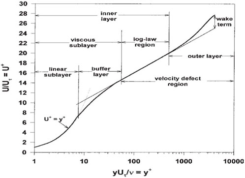
FIGURE 1. An illustration of the characteristics of the turbulent boundary layer.

The full paper is organized as follows. In the first section, the WMLES approach is outlined, followed by some typical validation results. In the second section, the model problems and results for TBLC on the turbulent flat plate boundary layer are presented. Finally, some conclusions with several findings are drawn.

The WMLES Approach and Validation

The present work mainly uses a wall-modelled large eddy simulation (WMLES) approach under a hybrid RANS-LES framework. The formulation starts from the governing Navier-stokes equation with the Favre average, which can be written in tensor form as in Eq. 1:

$\mathrm{e}\begin{array}{l}\frac{\partial \overline{\rho }}{\partial t}+\frac{\partial \overline{\rho }{\stackrel{\sim }{u}}_j}{\partial x_j}=0\\ \frac{\partial \overline{\rho }{\stackrel{\sim }{u}}_i}{\partial t}+\frac{\partial \overline{\rho }{\stackrel{\sim }{u}}_i{\stackrel{\sim }{u}}_j}{\partial x_j}+\frac{\partial \overline{p}}{\partial x_i}=\frac{\partial {\overline{\tau }}_{ij}}{\partial x_j}-\frac{\partial {\tau }_{ij}^{sgs}}{\partial x_j}\\ \frac{\partial \overline{\rho }\stackrel{\sim }{E}}{\partial t}+\frac{\partial \left(\overline{\rho }\stackrel{\sim }{E}+\overline{p}\right){\stackrel{\sim }{u}}_j}{\partial x_j}=\frac{\partial {\stackrel{\sim }{u}}_i{\stackrel{\sim }{\tau }}_{ij}}{\partial x_j}-\frac{\partial {\stackrel{\sim }{q}}_j}{\partial x_j}-\frac{\partial {\stackrel{\sim }{u}}_i{\tau }_{ij}^{sgs}}{\partial x_j}-\frac{\partial q_j^{sgs}}{\partial x_j}\end{array}(1)$

where $\left(\overline{•}\right)$ terms as a filter operation and $\left(\stackrel{\sim }{•}\right)$ terms as the Favre filter, and the subgrid-scale (SGS) stress tensor and the viscous tensor can be written as in Eq. 2:

$\begin{array}{l}{\tau }_{ij}^{sgs}=\overline{\rho }\left(u_i{u}_j-{\stackrel{\sim }{u}}_i{\stackrel{\sim }{u}}_j\right)\\ q_j^{sgs}=\overline{\rho }\left(u_{i}T-{\stackrel{\sim }{u}}_i\stackrel{\sim }{T}\right)\end{array}(2)$

For the traditional LES approach, the SGS stress tensor is often computed via a so-called LES SGS model. Alternatively, for the present WMLES simulation, the traditional Smagorinsky subgrid-scale (SGS) model in LES is replaced with a hybrid one, which can be read as in Eq. 3:

${\nu }_t=f_D\min \left\{\left.{\left(Ky\right)}^2,{\left(C_{SMAG}\Delta \right)}^2\right)\right\}\sqrt{2S_{ij}{S}_{ij}}(3)$

where $K=0.41$ is the von Karman’s constant and $C_{SMAG}=0.18$ is the SGS model constant, while the damping function is written as in Eq. 4:

$f_D=1-\exp \left(-y^{+}/A^{+}\right),y^{+}=\frac{y{u}_{\tau }}{v},A^{+}=26(4)$

and the length scale is defined as in Eq. 5:

$\Delta =\min \left({\Delta }_x,{\Delta }_y,{\Delta }_z\right)(5)$

The idea of the above WMLES approach can be regarded as using the Prandtl mixing length model near the wall; whereas, away from the wall, it switches over to the Smagorinsky SGS model. Actually, from the model equation (Eq. 1), one can see that when $Ky\ll C_{SMAG}\Delta$, the model turns out the Prandtl mixing length assumption, while when $Ky>C_{SMAG}\Delta$, the model turns out the Smagorinsky SGS model. The above model can also be regarded as an alternative to the classical LES with the advantage of reducing the stringent and Reynolds number-dependent grid resolution requirements of the classical wall-resolved LES.

From the formulation, in the WMLES approach, the RANS portion of the model is only activated in the inner part of the logarithmic layer (at y⁺< 15–20) and the outer part of the boundary layer is covered by a modified LES formulation. Since the inner portion of the boundary layer is responsible for the Reynolds number dependency of the LES model, the WMLES approach can be applied at the same grid resolution to an ever-increasing Reynolds number, which can be seen as illustrated in Figure 2. As shown in the figure, with the increasing Reynolds number, small-scale eddies confined within the viscous sublayer (VS) would get smaller and smaller such that it is necessary to avoid resolving them by using the WMLES approach. However, even at that, it is worth pointing out that the WMLES is still time-consuming as one kind of time-accurate computation method, and it is necessary to involve high-performance computing during the whole computation procedure [9].

FIGURE 2

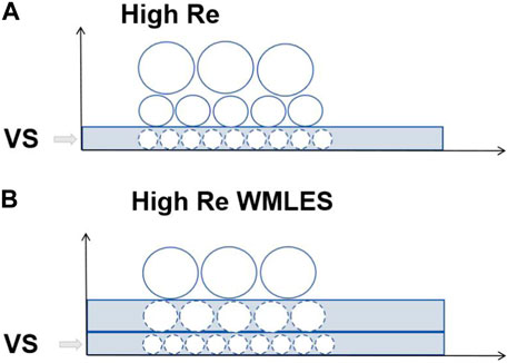
FIGURE 2. An illustration of the principle of the WMLES approach; (A) original LES; (B) WMLES.

The numerical considerations here include a central difference scheme (which has low numerical dissipation and dispersion), second-order time accuracy, and explicit time integration with dual time stepping. Besides, the two-dimensional VM method is introduced during the procedure for the inflow turbulence generation [10], which seems quite important for an LES or WMLES calculation for practical use.

In order to validate the efficiency of the present WMLES approach, numerical computation for an adverse-gradient flat plate case taken from [11] is performed, and the results are compared with those from the direct numerical simulation (DNS).

The flow condition is at $U_{\infty }=9m/s$ and $R{\mathrm{e}}_L=60000$. In Figure 3, the sketch of the computational grid for the case is shown, where a grid density $500\times 200\times 160$ is used to ensure enough dense grid density for the case. In Figure 4, typical results from the WMLES approach are given. From Figure 4A, one can see that the WMLES approach can predict the unsteady flow features very well and can give a very comprehensive detail of transient flow structures, which are coloured by velocity. Figure 4B shows that the present WMLES can give comparable results from DNS, which indicates that the WMLES can predict turbulence boundary layer very well, even with transition flow.

FIGURE 3

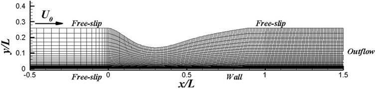
FIGURE 3. The sketch of the computational grid for the adverse gradient flat plate case.

FIGURE 4

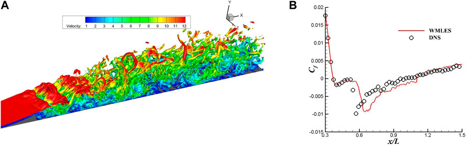
FIGURE 4. Numerical results for the adverse gradient flat plate case from the WMLES approach: (A) typical transient flow field; (B) comparison of the skin friction distribution with DNS.

Numerical Results of TBCL With Fluidic-Jet Actuator

Model Problems

In Figure 5, an illustration of the model problem of TBCL is shown. In the cases, a zero-gradient flat plate boundary layer with a length of 1.5 m is simulated as base flow, and six small span-wise rectangle slot holes are used to install fluidic-jet actuator arrays, which can take effect both for flow control in stream-wise and in span-wise. In the present study, all the fluidic-jet actuator arrays centre at $x=0.6m$, which have a slot width of $h=0.002m$, a slot length of $L=0.05m$, and a slot spacing of $d=0.012m$.

FIGURE 5

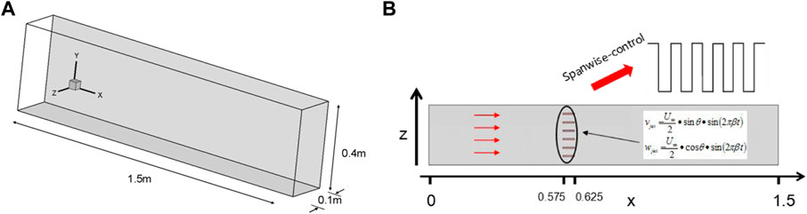
FIGURE 5. The model problem of TBCL: (A) set-up for the base flow and (B) set-up for the flow control.

In the simulation, three different control strategies are investigated (as shown in Table 1), which are named “W-control,” “V-control,” and “VW-control.” With such strategies, the fluidic-jet actuator can be modelled numerically by considering its specific application for the outer boundary layer control as in Eq. 6:

$\left\{\begin{array}{l}{v}_{jet}=\frac{U_{\infty }}{2}•\sin \theta •\sin \left(2\pi \beta t\right)\\ w_{jet}=\frac{U_{\infty }}{2}•\cos \theta •\sin \left(2\pi \beta t\right)\end{array}\right.(6)$

where $\theta$ is the injection angle, and $\beta$ is the actuating frequency. In the simulation, $\beta =20Hz$ is used for all simulations of TBLC of the turbulent flat plane.

TABLE 1

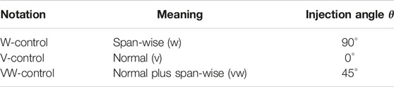
TABLE 1. Control strategies with fluidic-jet arrays.

The computational condition for the model problem can be found in Table 2, where both a low Reynolds number at ${\text{Re}}_{\tau }=470$ and a higher Reynolds number at ${\text{Re}}_{\tau }=4700$ are considered with the same free stream condition at $U_{\infty }=1.047m/s$ and the same inlet boundary layer thickness at $\delta =0.058m$.

TABLE 2

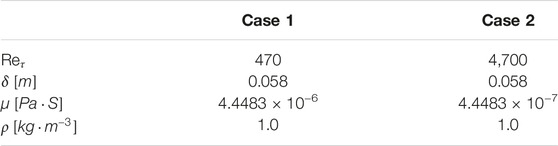
TABLE 2. Computational conditions for the model problem.

For the simulation, for the lower Reynolds number case, the grid with a total cell of around 13.9 million and grid density of $857\times 117\times 139$ is used to ensure enough dense grid density for the case, while for the higher Reynolds number case, the grid with a total cell of around 53.2 million and grid density of $1495\times 177\times 201$ is used.

Results for Low Reynolds Number Case at Re_τ = 470

In Figure 6, a typical transient flow field coloured by streamwise velocity, $u$, both for the base flow and the controlled flow (with “VW-control” strategy) at the same physical time is shown, where the Q-criterion = 200 is used to capture the large and small vortices structure of the turbulent boundary layer. From the results, one can conclude that a very clear and reasonable flow structure of the boundary layer of the present model problem can be obtained with the novel WMLES simulation.

FIGURE 6

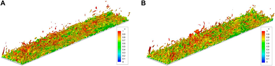
FIGURE 6. Transient flow field of (A) base flow and (B) controlled flow with VW-control at Re_τ = 470.

In Figure 7, mean velocity profiles taken at four different locations, $x=0.2$, $x=0.4$, $x=0.8$, and $x=1.2$, from the base flow are further shown and compared with the classical empirical correlation formulation. From the figure, one can also see that all the numerical profiles given by WMLES agree with the theoretical formulation very well, which validates the present numerical approach. Besides, from the figure, since all the numerical profiles are almost identical, it partly shows that a fully developed turbulent boundary layer is achieved in the case. In Figure 8, contours of vorticity magnitude at three typical locations, $y^{+}=1$, $y^{+}=10$, and $y^{+}=100$, are further shown. The streaks and streamwise vortices within the boundary layer are evident.

FIGURE 7

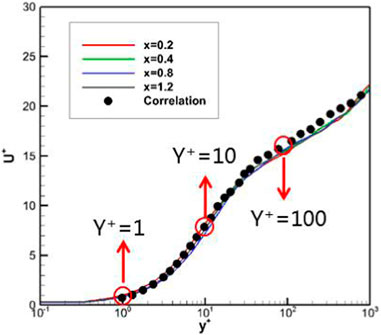
FIGURE 7. Velocity profiles at different locations for the base flow at Re_τ = 470.

FIGURE 8

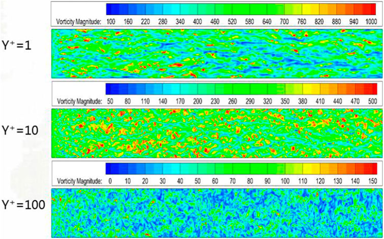
FIGURE 8. Contours of vorticity magnitude at three typical $y^{+}=1$ locations for the base flow at Re_τ = 470.

In Figure 9, the effect of the three different control strategies for drag reduction for the lower Reynolds number case is investigated, where the local drag reduction (DR) rate is defined in Eq. 7:

$dC{f}_w\left(\%\right)=\frac{C_f-C_{f,base}}{C_{f,base}}\times 100\%(7)$

FIGURE 9

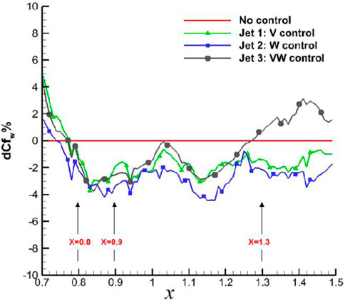
FIGURE 9. The effect of different controls for drag reduction for the lower Reynolds number case at Re_τ = 470.

From the result, an averaged local DR rate at 2%–3% for all types of flow control behind the actuator array can be achieved, and comparably, the “V-control” strategy can achieve a robust drag reduction downstream. In Figure 10, the contour of the average skin friction behind the jet actuator array is further shown. From the figure, one can see that different levels of drag reduction can be achieved through present control strategies via micro jet-actuators array.

FIGURE 10

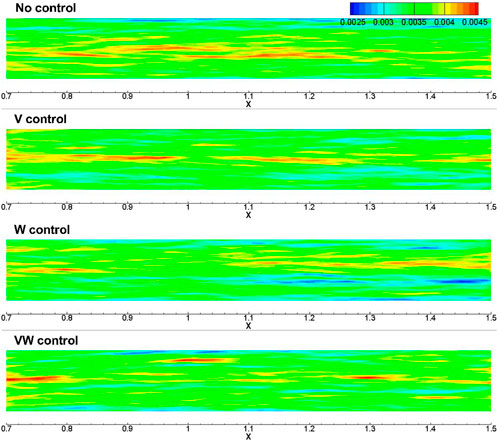
FIGURE 10. Comparison of average skin friction for the lower Reynolds number case between base flow and controlled flow at Re_τ = 470.

In order to analyse the origin targeting drag reduction with TBLC for these cases, in Figure 11 gives comparisons of the velocity profile at a typical location, $x=0.8$, between controlled flows and the base flow. From the figure, since the inner layer can be estimated to be around within $y^{+}=143$, one can find that for all these controlled cases, the inner layer would contribute to drag increase, while the outer layer would contribute to drag reduction. By contrast, the “V-control” strategy (marked as jet2) would achieve the smallest drag increase contribution from the inner layer. One can also conclude that since total drag reduction is achieved as shown in Figure 9, drag reduction is mainly contributed from the outer layer as we wanted.

FIGURE 11

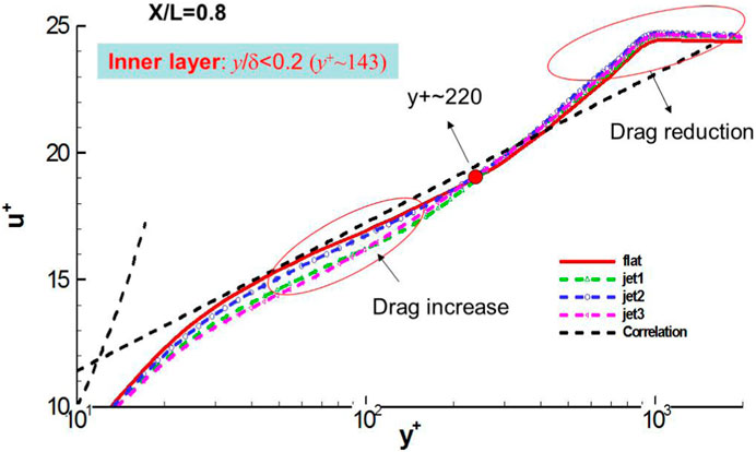
FIGURE 11. Comparison of the velocity profile at a typical location, x$=0.8$, between controlled flows and the base flow at Re_τ = 470.

Results for Higher Reynolds Number Case at Re_τ = 4700

Based on previous findings with different control strategies at the low Reynolds number case at Re_τ = 470, the “V-control” strategy is further investigated for TBLC of the higher Reynolds number case at Re_τ = 4700 in this section. In Figure 12, the comparison of the skin friction distribution between the base flow and the controlled flow is shown. It is found that, again, similar to the low Reynolds number case at Re_τ = 470, an obvious drag reduction will be achieved for the present higher Reynolds number case at Re_τ = 4700.

FIGURE 12

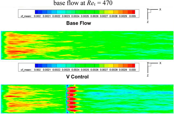
FIGURE 12. Comparison of average skin friction for the higher Reynolds number case between base flow and controlled flow at Re_τ = 4700.

In Figure 13, the local DR rate through the present “V-control” strategy is compared. It is found that compared with the low Reynolds number case at Re_τ = 470, a larger DR rate will be achieved at Re_τ = 4700. The maximum DR rate is more than 6%, and the average DR rate is approximately 5%.

FIGURE 13

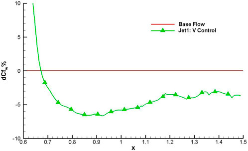
FIGURE 13. Effect of “V-control” for drag reduction for the higher Reynolds number case at Re_τ = 4700.

Mechanism Analysis for TBLC

As shown in Figure 14, a consequence of the control is a significant increase in the spanwise inter-streak distance, as determined from the spanwise two-point correlation, suggesting an increase in the scale of the near-wall streaks. Also, the control had a significant effect on the outer structures, in which the control weakened the streaky structure in the outer region.

FIGURE 14

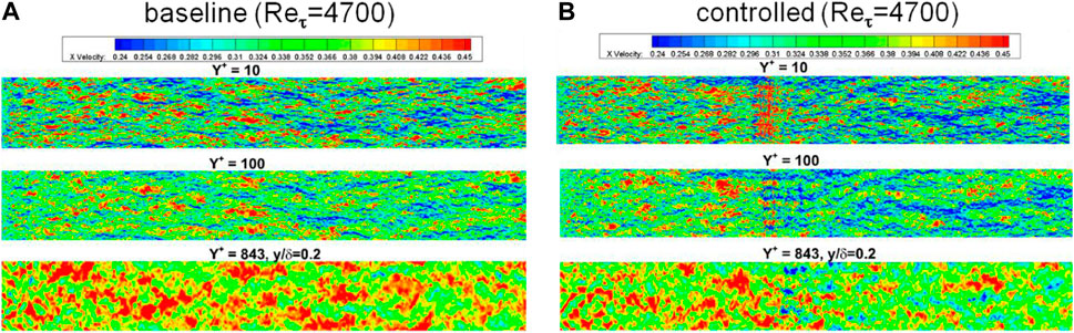
FIGURE 14. Typical footprints with and without “V-control” at Re_τ = 4700: (A) base flow; (B) controlled flow.

Figure 15 shows $u_{rms}^{\prime }$, $v_{rms}^{\prime }$, $w_{rms}^{\prime }$, and $<u^{\prime }{v}^{\prime }>$ plots with and without control. It can be seen that for all types of RMS, results from the controlled case are higher than those from the base flow. Therefore, it can be noticed that the control increases the RMS of velocities as well as the shear Reynolds stress. Besides, from the plot of ${\mathrm{u}}_{\text{rms}}^{\prime }$ without control, one can clearly find two peaks.

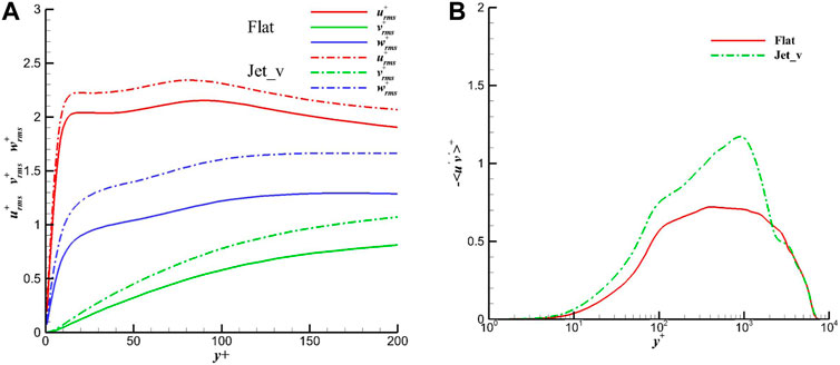
FIGURE 15

FIGURE 15. $u_{rms}^{\prime }$ , $v_{rms}^{\prime }$, $w_{rms}^{\prime }$, and $<u^{\prime }{v}^{\prime }>$ plots with and without “V-control” at Re_τ = 4700.

Figure 16 further shows the plots of pre-multiple energy spectra for streamwise velocity at x/c = 0.8 with and without control. Again, two peaks, where one is the inner peak and another is the outer peak, which generally occurs only for high Reynolds number flow, can be found for both cases. For the base flow case, the inner peak, associated with the streaks, is at around y⁺∼15 with λ⁺∼100, which corresponds to the small-scale motion; meanwhile, the outer peak is at around y⁺∼100 with λ⁺∼398. With control, the inner maximum in the spectra moves to y⁺∼39 with λ⁺∼170, and the outer maximum to y⁺∼794 with λ⁺∼630. As such, one can conclude that present TBLC using a “V-control” strategy with jet-actuators array can result in the outer peak moving forward and result in the intensity of energy spectral increasing as well.

FIGURE 16

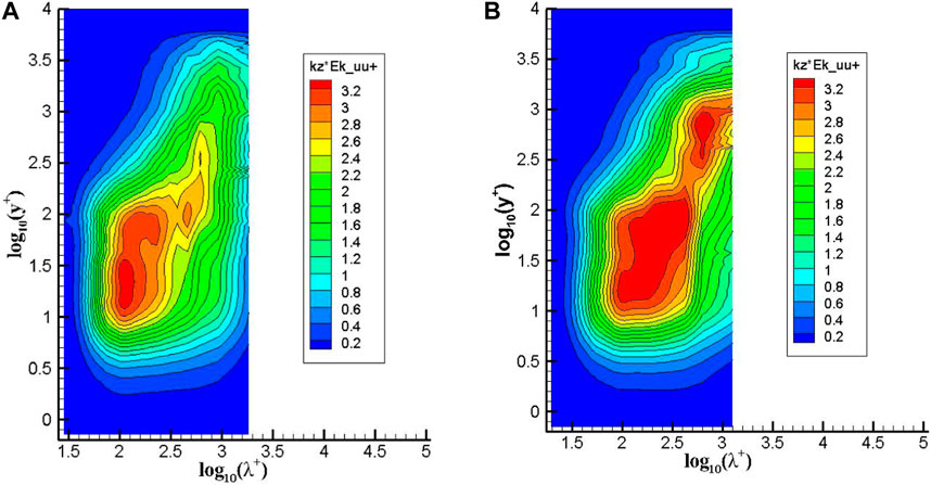
FIGURE 16. Pre-multiple energy spectral for the streamwise velocity at x/c = 0.8 with and without “V-control” at Re_τ = 4700.

In order to further investigate the mechanics for drag reduction of the outer layer TBLC for the flat plate boundary layer, a parallel dynamic mode decomposition (DMD) approach is introduced to implement the analysis for the whole flow field [12], where the DMD modes can be ordered according to their contribution to the energy and then examine which frequencies are most influential in terms of the energy contribution. Figure 17 shows energetically ordered distributions of DMD modes for both the canonical and controlled flows at the wall-normal plane $y^{+}=15$. As shown in the figure, approximately 40 modes are needed to recover around 78% of the energy. According to the plot of energy versus mode number, the difference between base flow and controlled flow is quite small. However, if we look at the plot of frequency versus amplitude for y⁺ = 15 as shown in Figure 18, with jet injection, a reduction in the frequency of most energetically relevant modes is found. It seems to suggest that the injection increases the importance of large-scale structures, possibly by the injection creating such structures in the inner layer.

FIGURE 17

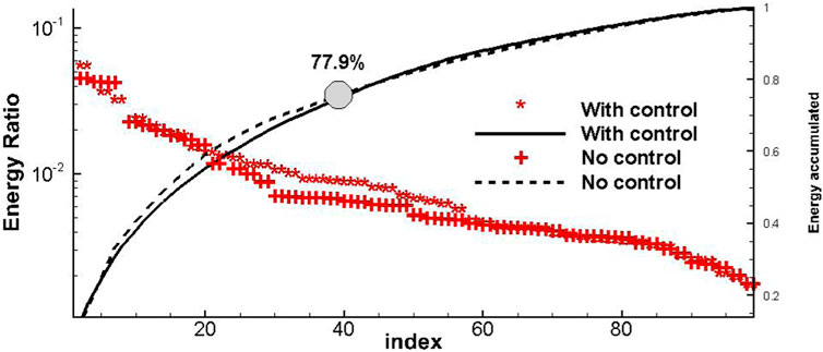
FIGURE 17. DMD mode distribution at y⁺ = 15 with and without “V-control” at Re_τ = 4700.

FIGURE 18

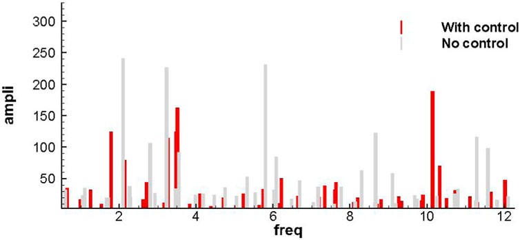
FIGURE 18. Frequency-amplitude plot at y⁺ = 15 with and without “V-control” at Re_τ = 4700.

Conclusion

A wall-modelled LES (WMLES) approach combined with high-performance computing is presented for the numerical investigation of outer-layer turbulent boundary layer control for drag reduction through micro fluidic-jet actuators. The studies are performed on the classical zero-gradient turbulent flat plate cases, in which three different control strategies named “W-control,” “V-control,” and “VW-control” are used and compared to study the effects of drag reduction under a low Reynolds number at Re_τ = 470 and a higher Reynolds number at Re_τ = 4700. Both the pre-multiplied spectral method and a parallel dynamic mode decomposition (DMD) method are introduced for analysis of the mechanism of the outer-layer boundary layer control for drag reduction. From the results, several conclusions can be drawn as follows.

First, it can be marked that the WMLES approach presented in this paper combined with high-performance computing is an efficient way for an accurate prediction of the turbulent flat plate boundary layer.

Second, for the model problem of TBLC based on the zero-gradient flat plate boundary layer, the Reynolds number is an important factor. For the lower Reynolds number at Re_τ = 470, an averaged local DR rate of around 2%–3% for all types of flow control behind the actuator array can be achieved, while for the higher Reynolds number at Re_τ = 4700, an average local DR rate of around 5%–6% can be achieved.

Finally, both the pre-multiplied spectral method and the DMD analysis indicate that the outer-layer TBLC with fluidic-jet actuator can increase the importance of large-scale structures of the boundary layer such that the structures in the inner layer would be affected. The obvious uplift of Reynolds shear stress and turbulent kinetic energy distribution may be the main mechanism for drag reduction.

Data Availability Statement

The original contributions presented in the study are included in the article/supplementary material, further inquiries can be directed to the corresponding authors.

Author Contributions

The first author, LL, conceptualization, methodology, numerical computation, and draft writing. The second author, JW, conceptualization, data analysis, and draft reviewer. The third author, YL, conceptualization, data analysis, and draft reviewer. The fourth author, ZT, conceptualization, numerical computation. All authors contributed to the article and approved the submitted version.

Funding

This work is partially supported by the China-EU Cooperation project, DRAGY (grant number: 690623), and the Shaanxi Key Research and Development Program (grant number: 2022ZDLGY02-07).

Conflict of Interest

The authors declare that the research was conducted in the absence of any commercial or financial relationships that could be construed as a potential conflict of interest.

References

1. Ma, HD. Drag Prediction and Reduction for Civil Transportation Aircraft. Mech Eng (2007) 29(2):1–8.

Google Scholar

2. Valero, E, Abbas, A, and Ferrer, E. Drag Reduction Technology Review. In: 2nd GRAIN2 Open Workshop on “Greening Aviation – A Global Challenge”. Xi’an, China: Chinese Aeronautical Establishment (2005).

Google Scholar

3. Reneaux, J. Overview on Drag Reduction Technologies for Civil Transport Aircraft. In: European Congress on Computational Methods in Applied Sciences and Engineering. Jyvaskyla, Finland: ECCOMAS (2004).

Google Scholar

4. Obert, E. Aerodynamic Design of Transport Aircraft. Delft, Netherlands: Delft University Press (2009).

Google Scholar

5. Zhang, JH, Li, BH, Wang, YF, and Jiang, N. Effects of Single Synthetic Jet on Turbulent Boundary Layer. Chin Phys B (2022) 31:074702. doi:10.1088/1674-1056/ac4bd0

CrossRef Full Text | Google Scholar

6. Schueller, M, Lipowski, M, Schirmer, E, Walther, M, Otto, T, Geßner, T, et al. Integration of Fluidic Jet Actuators in Composite Structures. In: Proc. SPIE 9431, Active and Passive Smart Structures and Integrated Systems. San Diego, California, United States: SPIE (2015).943113

CrossRef Full Text | Google Scholar

7. Abbas, A, Bugeda, G, Ferrer, E, Fu, S, Periaux, J, Pons-Prats, J, et al. Drag Reduction via Turbulent Boundary Layer Flow Control. Sci China Technol Sci (2017) 60(9):1281–90. doi:10.1007/s11431-016-9013-6

CrossRef Full Text | Google Scholar

8. Pierre, R, Martin, S, and Michael, AL. A Review of Turbulent Skin-Friction Drag Reduction by Near-Wall Transverse Forcing. Prog Aerospace Sci (2021) 123:100731.

Google Scholar

9. Li, L, Wu, JS, Liang, YH, and Tian, ZD. A Wall-Modeled Large Eddy Simulation Approach Based on Large Scale Parallel Computing for Post Stall Flow Over an Iced Airfoil. J Northwest poly-technical Univ (2023) 41(5):1–10.

CrossRef Full Text | Google Scholar

10. Zhou, L, Yang, QS, Yan, BW, Wang, J, and Van Phuc, P. Review of Inflow Turbulence Generation Methods With Large Eddy Simulation for Atmospheric Boundary Layer. Eng Mech (2020) 37(5):15–25. doi:10.6052/j.issn.1000-4750.2019.06.0340

CrossRef Full Text | Google Scholar

11. Wissink, J, and Rodi, W. Direct Numerical Simulations of Transitional Flow in Turbomachinery. J Turbomach (2006) 128:668–78. doi:10.1115/1.2218517

CrossRef Full Text | Google Scholar

12. Tan, WW, Bai, JQ, and Tian, ZD. Parallel Dynamon for Rayleigh-Taylor Instability Flows. In: Asia-Pacific International Symposium on Aerospace Technology. Chendu, China: Springer (2019).

Google Scholar