Abstract
This work introduces Pontryagin Neural Networks (PoNNs), a specialised subset of Physics-Informed Neural Networks (PINNs) that aim to learn optimal control actions for optimal control problems (OCPs) characterised by integral quadratic cost functions. PoNNs employ the Pontryagin Minimum Principle (PMP) to establish necessary conditions for optimality, resulting in a two-point boundary value problem (TPBVP) that involves both state and costate variables within a system of ordinary differential equations (ODEs). By modelling the unknown solutions of the TPBVP with neural networks, PoNNs effectively learn the optimal control strategies. We also derive upper bounds on the generalisation error of PoNNs in solving these OCPs, taking into account the selection and quantity of training points along with the training error. To validate our theoretical analysis, we perform numerical experiments on benchmark linear and nonlinear OCPs. The results indicate that PoNNs can successfully learn open-loop control actions for the considered class of OCPs, outperforming the commercial software GPOPS-II in terms of both accuracy and computational efficiency. The reduced computational time suggests that PoNNs hold promise for real-time applications.
Introduction
Optimal control theory has been a major area of interest in various scientific fields throughout the last century. Optimal Control Problems (OCPs) are fundamental in many disciplines, leading to the development of numerous numerical methods aimed at optimising cost functions that are central to OCPs. In general, OCPs can be addressed using two main approaches: direct methods and indirect methods [1].
Direct methods involve discretising the continuous states and controls to transform the continuous problem into a Nonlinear Programming (NLP) problem [2–4]. This transformation results in a finite constrained optimisation problem solvable by various algorithms designed to find local minima, such as trust-region methods [5]. Direct methods have been applied to a wide range of OCPs, particularly in the aerospace sector (e.g., [6–9]). However, the general NLP problem is considered NP-hard, meaning that the computational time required to find the optimal solution cannot be predetermined and can be substantial. This uncertainty in convergence time can undermine the reliability of these methods, especially in real-time applications.
To address these challenges, researchers have explored transforming OCPs from non-convex formulations into convex optimisation problems [10, 11]. Convex problems are computationally tractable because their associated numerical algorithms guarantee convergence to a global optimum in polynomial time. This approach involves applying convexification techniques to reformulate the optimal guidance problem into a convex one. Such methodologies have been successfully used in various aerospace applications, including planetary landing [10, 11], atmospheric entry guidance [12, 13], rocket ascent guidance [14], and low-thrust trajectory optimisation [15].
Indirect methods, on the other hand, derive first-order necessary conditions by applying the Pontryagin Minimum Principle (PMP) or the calculus of variations. These necessary conditions lead to a Two-Point Boundary Value Problem (TPBVP) that involves state and costate variables, which must be solved numerically. Available numerical methods for indirect approaches include single and multiple shooting methods [16, 17], orthogonal collocation [18], and pseudospectral methods [19]. The commercial software GPOPS-II, based on the work presented in [20], represents the current state-of-the-art. While the indirect method guarantees an optimal solution, solving the TPBVP can be challenging due to the sensitivity of the solution to initial guesses, particularly for costate variables that lack physical interpretation. Although direct methods may not always yield optimal solutions, they are generally easier to compute and are widely used in the scientific community.
In principle, these two approaches can be combined. For instance, a solution obtained via a direct method can serve as an initial guess for an indirect method, potentially refining the solution and ensuring optimality.
In this work, we addressed a class of OCPs with integral quadratic cost functions by applying the PMP and solving the resulting TPBVP using a specialised Physics-Informed Neural Network (PINN) framework known as the Extreme Theory of Functional Connections (X-TFC) [21–24]. In our approach, PINNs are tailored and trained to learn optimal control actions by enforcing the physics constraints represented by the TPBVP arising from the application of the PMP. We refer to these specialised PINNs as Pontryagin Neural Networks (PoNNs).
The main contributions and objectives of this paper are threefold: 1) to demonstrate the feasibility of using PINN-based frameworks to directly learn TPBVP solutions and, consequently, open-loop optimal control with high accuracy and low computational time; 2) to provide an estimate of the generalisation error associated with the proposed methodology; and 3) to compare the performance of PoNNs with the commercial software GPOPS-II [20].
Physics-Informed Neural Networks (PINNs) are a machine learning framework that incorporates physical laws, expressed as differential equations (DEs), into the training of neural networks (NNs) by including them as regularisation terms in the loss function [25]. In classical PINNs, the DE constraints are included in the loss function alongside the residuals computed within the domain. However, this approach has a significant drawback: it requires the simultaneous satisfaction of the DEs and their associated boundary conditions (BCs) or initial conditions (ICs) during training, which can complicate the optimisation process [26].
The X-TFC framework enhances the classical PINN approach by using Constrained Expressions (CEs) from the Theory of Functional Connections (TFC) [27]. The general form of a CE is given bywhere is the unknown function to be approximated, is the CE, is a functional that analytically satisfies the given linear constraints, and projects the free function —which exists over the constraints—onto the space of functions that vanish at the constraints [28].
TFC is a functional interpolation technique applicable to various mathematical problems, including the solution of differential equations (DEs) [29] and the addressing of OCPs via the PMP approach. While the original TFC employs linear combinations of orthogonal polynomials as the free function, this can lead to computational challenges, especially for large-scale partial differential equations (PDEs), due to the curse of dimensionality [29]. To mitigate these issues, PINN TFC-based methods use neural networks as the free function. Specifically, X-TFC employs Extreme Learning Machines (ELMs), which are shallow neural networks with random features, also known as Random Projection Networks.
X-TFC has been successfully applied to solve integro-differential equations [30] with applications in rarefied gas dynamics [31, 32] and radiative transfer equations [33]. It has also been used for stiff systems of ODEs in nuclear reactor dynamics [34] and stiff chemical kinetics [35], as well as inverse problems for system identification [36, 37] and parameter estimation in epidemiological models [38]. Additionally, X-TFC has been applied to a class of OCPs for aerospace applications using both indirect methods [39, 40] and the Bellman Optimality Principle [41].
This paper is organised as follows. First, we describe how PoNNs are constructed and trained to learn control actions for the class of OCPs with integral quadratic cost functions. We then provide an upper bound estimate on the generalisation error of PoNNs in learning solutions for the considered OCP class, in terms of training error and the number and selection of training points. Two benchmark OCPs—one linear and one nonlinear—are used to demonstrate the effectiveness of PoNNs in learning optimal control actions and to validate our theoretical findings. We also compare the performance of PoNNs with the commercial software GPOPS-II. Finally, we present our conclusions.
Materials and Methods
Pontryagin Neural Networks (PoNNs) are a specialised class of Physics-Informed Neural Networks (PINNs) designed to solve Optimal Control Problems (OCPs) through the application of the Pontryagin Minimum Principle (PMP). In this study, we focused on OCPs characterised by integral quadratic cost functions.
The term Pontryagin Neural Networks (PoNNs) was introduced to succinctly describe PINNs that are tailored to learn optimal control strategies via PMP [39]. The unknown solutions of the resulting Two-Point Boundary Value Problem (TPBVP), specifically the states and costates, are represented using a PINN framework based on the Extreme Theory of Functional Connections (X-TFC), developed by the authors.
In PINN TFC-based frameworks, unknown solutions of differential equations are modelled using Constrained Expressions (CEs) from the Theory of Functional Connections (TFC), with neural networks serving as free functions. When Deep Neural Networks (DNNs) are employed as free functions, the framework is referred to as Deep-TFC [28], where gradient-based optimisation methods like the ADAM optimiser [42] or the L-BFGS optimiser [43] are used to adjust the parameters.
Alternatively, when shallow neural networks trained using the Extreme Learning Machine (ELM) algorithm [44] are used as free functions, the framework is known as Extreme-TFC (X-TFC) [21]. The ELM algorithm initialises the input weights and biases randomly, keeping them fixed during training, which means that only the output weights are optimised [44]. This approach allows for robust and fast training using least-squares methods.
For linear differential equations, X-TFC optimises the free-function parameters (i.e., the neural network output weights) using a single-pass least-squares method. In the case of nonlinear differential equations, iterative least-squares procedures are required to optimise the parameters, as detailed in [21].
This section outlines the design and training process of PoNNs to learn optimal control actions for the class of OCPs under consideration. Additionally, following Refs. [22, 45], we derive an estimate for the upper bounds on the generalisation error of PoNNs in learning solutions for this class of OCPs.
A general OCP can be formulated as:
Here, represents the states that may be subject to path constraints, denotes the controls that may be subject to inequality constraints, and defines the terminal conditions. The cost function includes both a Meyer term (dependent on the final state and time) and a Lagrangian term (dependent on the states and controls over time). The final time can be fixed or a function of the initial states (e.g., in time-free problems). Applying PMP transforms the OCP into the following TPBVP:
with , where is the Hamiltonian of the problem, and , , , with being the costates. Equation 2 encompasses all possible transversality conditions for unconstrained OCPs, although the specific conditions applied depend on the problem at hand. Further details are available in [46, 47].
In this work, we focus on unconstrained OCPs with a fixed final time and a fixed final state, leading to the following TPBVP:
Here, , , , , , and are all -dimensional vectors, with being the number of states. Equation 3 is well-posed and can be expressed compactly as:where and . We assume that is globally Lipschitz continuous, meaning that there exists a constant (independent of ) such that:
To apply the X-TFC algorithm to solve Equation 4, we need to specify the training set and define the residuals. Considering the time domain , we selected the training set based on suitable quadrature points, such as those corresponding to a composite Gauss quadrature rule or randomly selected points, as suggested in Ref. [45]. The training points are defined as:
Using the constrained expressions, we approximate the solution of Equation 4. The states are approximated by:
The costates are approximated by:whereand
In these expressions, and are the input weights and biases, respectively, and is the number of hidden neurons. Since and are single-layer neural networks with random features, the weights and biases are randomly initialised and remain fixed during training; only the output weights are optimised. Notably, and constitute the PoNNs.
We define the residuals as:wherewith
To train the PoNNs and learn the unknown solutions, we minimise the following vector-valued loss function:
With the loss function defined, the X-TFC algorithm is fully specified and can be executed to learn the solution of the TPBVP in Equation 4 resulting from the application of the PMP. The learnt PoNNs are denoted as , where are the optimised output weights obtained from training.
If the loss function in Equation 7 is linear, it simplifies to a system of linear algebraic equations of the form , which can be solved using a single-pass least-squares method. For nonlinear loss functions, an iterative least-squares procedure is necessary, as described in [21].
Figure 1 illustrates the flowchart for learning optimal control problem solutions using the proposed PoNNs.
FIGURE 1
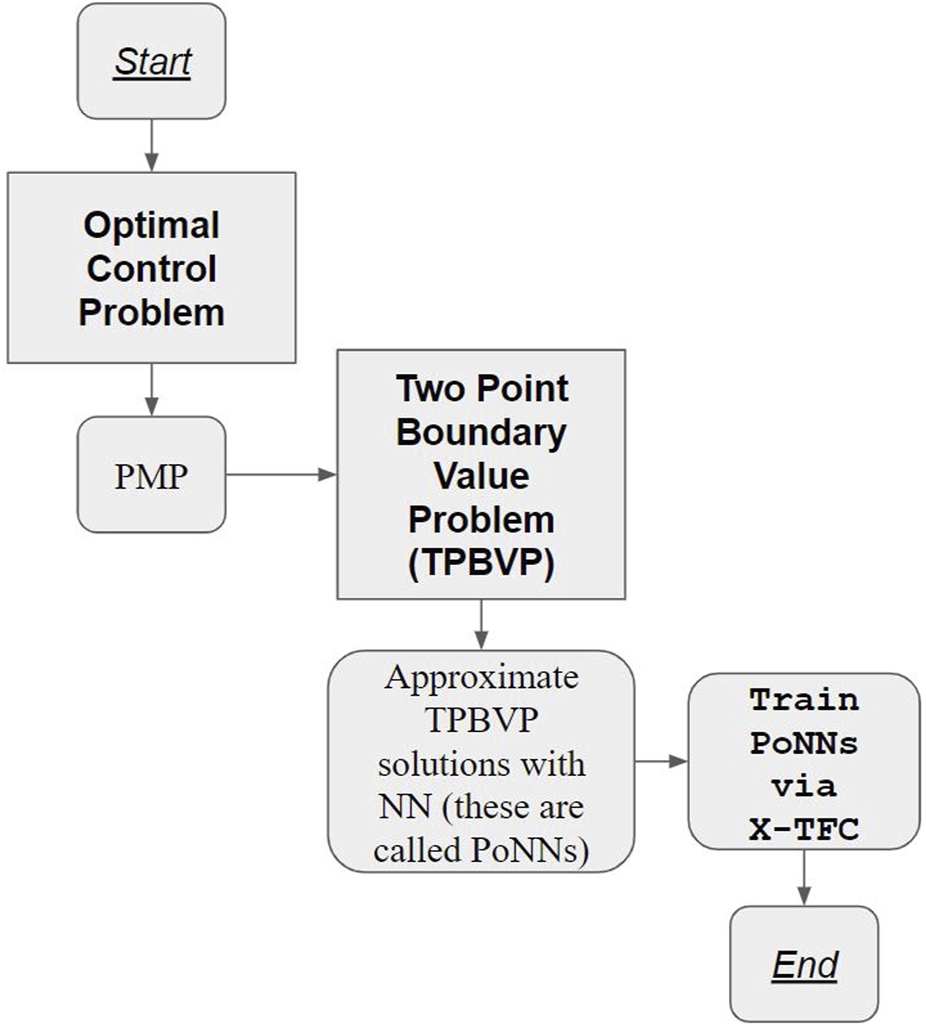
Flowchart for learning optimal control problem solutions using the proposed PoNNs.
Estimation of the Generalisation Error
We are interested in estimating the generalisation error for X-TFC, which is defined aswhere , according to [45] and references therein, is the error emerging from approximating the true solution, , via X-TFC, within the domain . We estimate the generalisation error in terms of the training error defined as,which is computed a posteriori once the training is completed.
According to Ref. [45], we also need the following assumptions on the quadrature error: for any function , the quadrature rule corresponding to the quadrature weights at points , with , satisfies,where and different order quadrature rules can be used (details can be found in [45]). The estimate of the generalisation error for X-TFC is given by the following theorem.
Let be the unique classical solution of the general TPBVP (Equation 4), resulting from the PMP application to Equation 1, with the dynamics satisfying Equation 5. Let be the solution approximated via X-TFC, corresponding to the loss function (Equation 7). Then, the generalisation error (Equation 8) can be estimated as,where is given by Equation 9, the constant is given by,andwhich is a function of the residuals ,Alsowhich is a positive constant depending on the number of training points, the quadrature scheme used, and the residuals evaluated on the training points [45].
Proof
Using the definitions of the residuals (Equation 6), and the system (Equation 4), we can verify that the error satisfies the following equation,Here, we have denoted for convenience of notation. Multiplying both sides of the system (Equation 11) by yieldswhere is the inner product. That is,By leveraging on the following inequality , Equation 12 is bounded by,By Equation 5, we have the following,Rearranging we get,Integrating the above inequality over for any , we obtain,where,with because of the CE.
Also,since and . Thus,Applying the integral form of the Grönwall’s inequality to the above, we getIntegrating over in ,That is,Thus,Finally,where,This completes the proof.
The estimate (Equation 10) indicates that the generalisation error when training PoNNs is small under several conditions. The training error for the PoNN must be reasonably small (e.g., ). Moreover, the training error can only be computed a posteriori, as we have no prior control over it. The error associated with the training points depends on the choice and the number of training points as well as on the training constant . The latter also depends on the residual of the PoNN, , and thus, indirectly, on the number of training points . That is, needs to be large enough so that . The constant also depends on the architecture of the underlying PoNN. The evaluation depends on the features of the governing DEs, and the collocation of the training points cannot be worked out in the setting of Theorem 1 [48]. The constant encodes the stability of the DEs and depends on both the exact (unknown) solution and the trained PoNN, , that needs to be bounded. For OCPs with fixed final state, the term can be computed for linear problems. In this case it is related to the transition matrix. For nonlinear problems, cannot be known. If it were known, the main limitation of the indirect method for solving OPCs would be removed (e.g., the sensitivity of the guess on the costates initial value). Moreover, if this were the case, we would solve the problem with a perfect shooting method. However, if the domain is compact, we can guarantee that if the other terms in the are small enough, then will also be small enough (e.g., ). Therefore, PoNN will generalise well the unknown solution (e.g., ). Conversely, if the OCPs have a free final state, in the TPBVP (Equation 4) we will have the condition instead of . In this case, the condition on the costate at the final time can be considered as an initial condition for a backward problem, and thus the TPBVP is tackled as a first-order Initial Value Backward Problem.
The main point of the estimate (Equation 10) is to provide an upper bound of the generalisation error in terms of the training and quadrature errors, regardless of the choice of the PoNN architecture. The estimate (Equation 10) holds for any expansion of , including NNs (of any type). There is no guarantee that the training error will be small if NNs are used to approximate . However, it can be expected that if the DE is stable and the training points collocation scheme is accurate (e.g., there is some control over and ), the training error will be small, leading to a small generalisation error. Nevertheless, for some PoNN architectures, where the training error was small, but and were not (e.g., for high and/or not enough training points ), the overall estimate would not be small enough (e.g., would not be ). In this scenario, PoNN would not generalise well the unknown solution .
Results
To test our theoretical findings, two benchmark OCPs are studied: 1) linear hypersensitive Feldbaum problem and 2) nonlinear hypersensitive Feldbaum problem.
All the selected problems are coded in MATLAB 2022a and run on an Intel Core i7 - 9700 CPU PC with 64 GB of RAM.
Problem 1: Linear Hypersensitive Feldbaum Problem
The problem considered here is a linear hypersensitive OCP taken from [49, 50], also known as the Hypersensitive Feldbaum Problem (HFP). The problem is cast as follows:The resulting TPBVP after the PMP application is,
The analytical solution is available and provided in [50].
For the PoNN algorithm, we will use the following hyperparameters in all cases: Gaussian activation function, input and bias are sampled from . It should also be noted that the computed times of execution are reported on their own scale.
In Figure 2, the two plots on the left show the analytical, PoNNs, and GPOPS-II solutions. On the plots on the right, the absolute errors of PoNNs and GPOPS-II at the points when compared with the analytical solution are shown. In the first row for the State variable, in the second row for the Control one. We used , which was trained on 100 randomly generated points. GROPS-II used points.
FIGURE 2
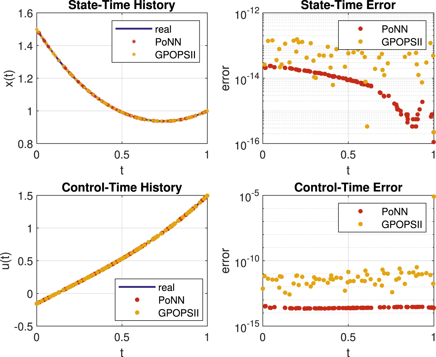
Computed solutions and absolute errors for the linear test problem.
Figure 3 shows the comparison with the results obtained by GPOPS-II. We report convergence results when increasing the number of neurons fixing and using exactly the points given by the (adaptive) procedure of GROPS-II. We note that in the result, the error made by the commercial software is strongly affected by an anomalous value obtained at the final time, see Figure 2.
FIGURE 3
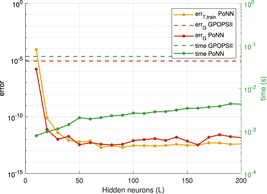
Convergence of the PoNN algorithm when increasing the number of neurons , comparison with the result obtained by GPOPS-II. The training points are fixed and coincide with those used by GPOPS-II .
In Figure 4 we report the obtained results by applying our algorithm. It should be noted that the computation time can be affected by the (machine precision) lower rank.
FIGURE 4
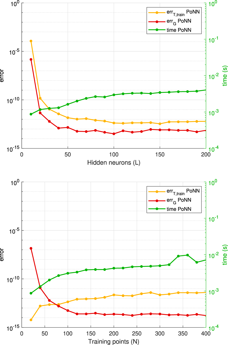
Convergence history for the application of the PoNN method to the linear problem. At the top, is the case with fixed training points, at the bottom, the one with fixed number of neurons.
The numerical tests confirm the theoretical findings. The comparison against GPOPS-II shows that PoNNs outperform GPOPS-II both in terms of accuracy and computational time. It should be noted that GPOPS-II was run with the default options, i.e., we did not require machine-level accuracy. In all cases, PoNNs achieve the machine-level accuracy with a lower computational time than GPOPS-II. Moreover, this last only reaches a default accuracy. Therefore, if GPOPS-II were pushed to machine level accuracy the gap in computation time would be higher. This assesses the superiority of PoNNs in terms of both accuracy and computation time.
Problem 2: Nonlinear Hypersensitive Feldbaum Problem
The problem considered here is a nonlinear version of the HFP considered before. The problem is formulated as follows:The resulting TPBVP after the PMP application is,The analytical solution is not available. Thus, to compute the error, we estimate it over the residual on the training points. To validate the accuracy of the target PoNN solution, we have compared it with the one generated with GPOPS-II and also evaluated its residuals. In all simulations, the hyperparameters used are: Gaussian activation function, input and bias sampled from .
In Figure 5 we report state and control time evaluations on training points. Training is performed on randomly sampled points with hidden neurons for the PoNN method, while GPOPS uses training points.
FIGURE 5
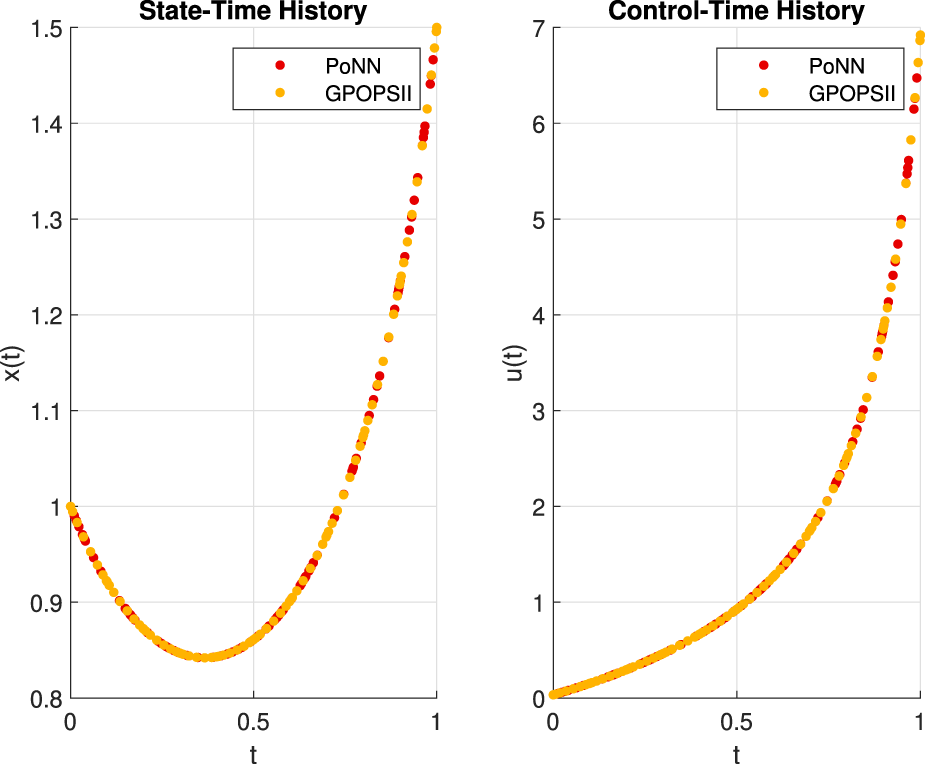
Visual comparison of the numerical solution. PoNN on N = 100 random training points. GPOPS uses 86 points for training.
In Figure 6 we show the residuals obtained when the parameters are increased: at the top, the number of neurons is increased while the number of training points (randomly generated) is fixed at ; at the bottom the number of training points is increased while the number of neurons is fixed at .
FIGURE 6
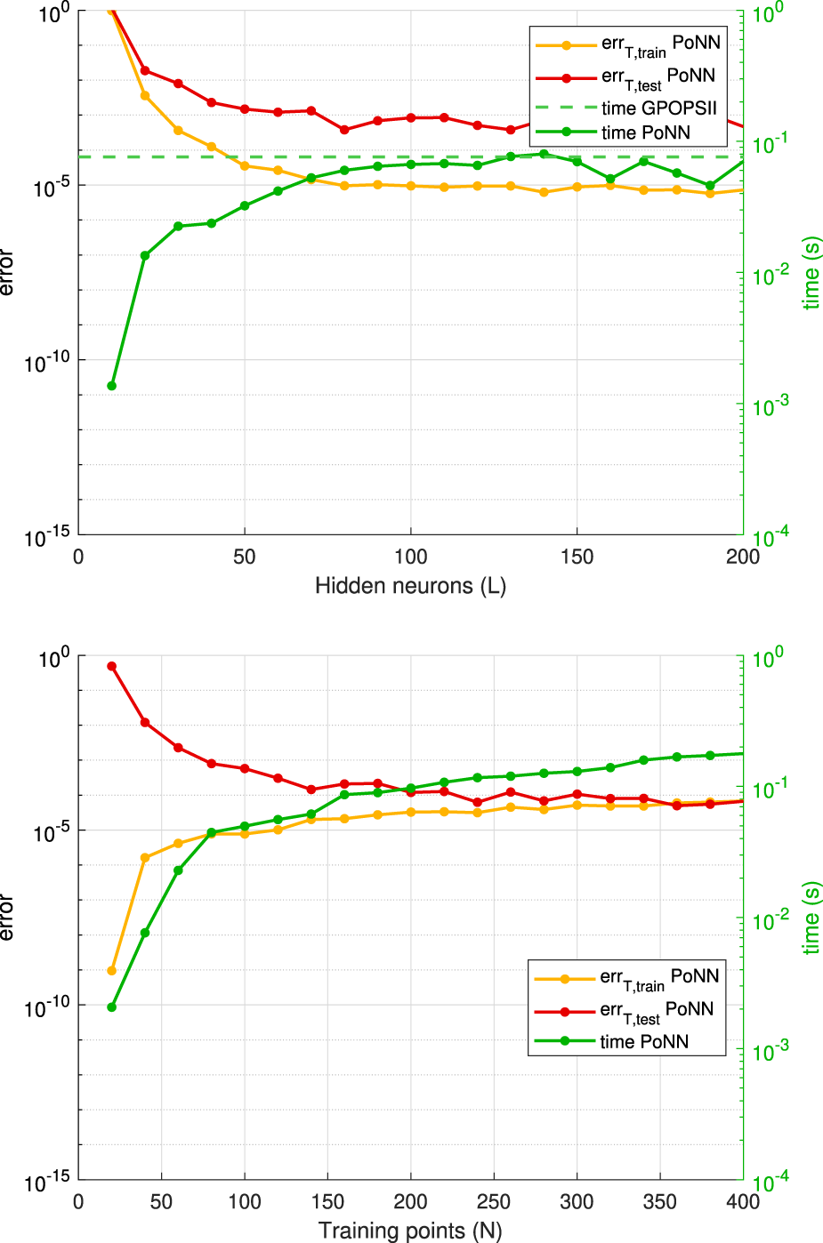
Convergence and stability results. On the ordinate is the computed residual, which is taken as an estimate of the overall error.
Even for the nonlinear case, the numerical tests confirm the theoretical findings.
Discussion
In this paper, we have introduced PoNNs and used them to learn the solutions to OCPs with integral quadratic cost, which were tackled via the indirect method.
The proposed approach can be applied to all research fields where OCPs with integral quadratic cost must be solved. The low computational time makes PoNNs attractive for real-time applications.
We have derived upper bounds on the generalisation error, in terms of the training error and number and choice of training points, of PoNNs in learning OCP solutions. The theoretical results are validated with numerical experiments on a benchmark linear and a benchmark nonlinear OCPs. Furthermore, the results are compared with those generated with the commercial software GPOPS-II. PoNNs outperform the GPOPS-II both in terms of accuracy and computation time. It should be noted that the GPOPS-II was run with the default options, i.e., we did not require machine-level accuracy. In all cases, PoNNs reach a higher level of accuracy with a lower computation time than GPOPS-II reaches the default accuracy. Therefore, if GPOPS-II were pushed to machine level accuracy the gap in computation time would be higher. This assesses the superiority of PoNNs in terms of both accuracy and computation time.
It should also be noted that PoNNs are not (at all) optimised as GPOPS-II is. For instance for a more complex problem, where a domain decomposition may be required to achieve better performance, GPOPS-II will most likely achieve better results than PoNNs. Therefore, leveraging on this paper’s results (in particular the superiority of PoNNs on simple benchmark problems such as those considered in this manuscript), work is in progress to optimise PoNNs. In particular, the authors are working on adaptive domain-decomposition techniques.
A different and complementary approach to solving OCP comes from the application of the Bellman Principle of Optimality (BPO). The latter provides the necessary and sufficient conditions for optimality which yields in writing the so-called Hamilton-Jacobi-Bellman Equation (HJB) equation. The HJB is a nonlinear PDE that plays a crucial role in the optimal control theory. The solution of the HJB equation is the value function in all the time-state space. The value function represents the optimal cost-to go for a dynamical system with an associated cost function. Once the value function is known, the optimal control is also known as it is the gradient of the value function to the state variables. This means that, if we learn the solution of the HJB equation in the entire time-state space, we would also consequentially learn the optimal control actions in the entire time-state space in a closed-loop fashion. However, since it is not trivial and, in many cases, it is most likely impossible to find an analytical solution to the HJB equation, one has to resort to numerical methods. The main issue in solving HJB PDEs is that the spatial complexity of the problem increases exponentially with respect to the number of dimensions of the system. Thus the majority of the state-of-the-art numerical methods to tackle PDEs struggle to solve the HJB equation. The reason why the HJB equation should be addressed in the future is that, unlike the PMP, which provides just a necessary condition for the optimality and results in an open-loop locally optimal trajectory, the HJB equation can guarantee a necessary and sufficient condition for the optimality and provides a closed-loop solution [51, 52].
Statements
Data availability statement
The raw data supporting the conclusions of this article will be made available by the authors, without undue reservation.
Author contributions
ES and FC contributed to conception and design of the study. ES and DD wrote the first draft of the manuscript. All authors contributed to the article and approved the submitted version.
Funding
The author(s) declare that financial support was received for the research, authorship, and/or publication of this article. FC was partially supported by PRIN 2022 PNRR P2022WC2ZZ “A multidisciplinary approach to evaluate ecosystems resilience under climate change” and by PRIN 2022 2022N3ZNAX “Numerical Optimization with Adaptive Accuracy and Applications to Machine Learning.”
Acknowledgments
FC and DD are members of the INdAM research group GNCS and were partially supported by GNCS-INdAM; this support is gratefully acknowledged.
Conflict of interest
The authors declare that the research was conducted in the absence of any commercial or financial relationships that could be construed as a potential conflict of interest.
References
1.
RaoAV. A Survey of Numerical Methods for Optimal Control. Adv Astronautical Sci (2009) 135:497–528.
2.
DarbyCLHagerWWRaoAV. An hp-Adaptive Pseudospectral Method for Solving Optimal Control Problems. Optimal Control Appl Methods (2011) 32:476–502. 10.1002/oca.957
3.
FahrooFRossIM. Direct Trajectory Optimization by a Chebyshev Pseudospectral Method. J Guidance, Control Dyn (2002) 25:160–6. 10.2514/2.4862
4.
RossIMFahrooF. Pseudospectral Knotting Methods for Solving Nonsmooth Optimal Control Problems. J Guidance, Control Dyn (2004) 27:397–405. 10.2514/1.3426
5.
ByrdRHGilbertJCNocedalJ. A Trust Region Method Based on Interior Point Techniques for Nonlinear Programming. Math programming (2000) 89:149–85. 10.1007/pl00011391
6.
JosselynSRossIM. Rapid Verification Method for the Trajectory Optimization of Reentry Vehicles. J Guidance, Control Dyn (2003) 26:505–8. 10.2514/2.5074
7.
GrahamKFRaoAV. Minimum-Time Trajectory Optimization of Multiple Revolution Low-Thrust Earth-Orbit Transfers. J Spacecraft Rockets (2015) 52:711–27. 10.2514/1.a33187
8.
MillerATRaoAV. Rapid Ascent-Entry Vehicle Mission Optimization Using Hp-Adaptive Gaussian Quadrature Collocation. In: AIAA Atmospheric Flight Mechanics Conference, Grapevine, Texas, January 9–13, 2017 (2017), 0249.
9.
JiangXLiSFurfaroR. Integrated Guidance for Mars Entry and Powered Descent Using Reinforcement Learning and Pseudospectral Method. Acta Astronautica (2019) 163:114–29. 10.1016/j.actaastro.2018.12.033
10.
AcikmeseBPloenSR. Convex Programming Approach to Powered Descent Guidance for Mars Landing. J Guidance, Control Dyn (2007) 30:1353–66. 10.2514/1.27553
11.
BlackmoreLAcikmeseBScharfDP. Minimum-Landing-Error Powered-Descent Guidance for Mars Landing Using Convex Optimization. J guidance, Control Dyn (2010) 33:1161–71. 10.2514/1.47202
12.
WangZGrantMJ. Constrained Trajectory Optimization for Planetary Entry via Sequential Convex Programming. In: AIAA Atmospheric Flight Mechanics Conference, Washington, DC, June 13–17, 2016 (2016). p. 3241.
13.
WangZGrantMJ. Autonomous Entry Guidance for Hypersonic Vehicles by Convex Optimization. J Spacecraft Rockets (2018) 55:993–1006. 10.2514/1.a34102
14.
ZhangKYangSXiongF. Rapid Ascent Trajectory Optimization for Guided Rockets via Sequential Convex Programming. Proc Inst Mech Eng G: J Aerospace Eng (2019):0954410019830268.
15.
WangZGrantMJ. Minimum-Fuel Low-Thrust Transfers for Spacecraft: A Convex Approach. IEEE Trans Aerospace Electron Syst (2018) 54:2274–90. 10.1109/taes.2018.2812558
16.
KellerHB. Numerical Solution of Two Point Boundary Value Problems, 24. SIaM (1976).
17.
StoerJBulirschR. Introduction to Numerical Analysis, 12. Springer Science and Business Media (2013).
18.
OhSLuusR. Use of Orthogonal Collocation Method in Optimal Control Problems. Int J Control (1977) 26:657–73. 10.1080/00207177708922339
19.
FahrooFRossI. Trajectory Optimization by Indirect Spectral Collocation Methods. In: Astrodynamics Specialist Conference, Denver, CO, August 14–17, 2000 (2000). p. 4028.
20.
PattersonMARaoAV. Gpops-ii: A Matlab Software for Solving Multiple-Phase Optimal Control Problems Using hp-Adaptive Gaussian Quadrature Collocation Methods and Sparse Nonlinear Programming. ACM Trans Math Softw (TOMS) (2014) 41:1–37. 10.1145/2558904
21.
SchiassiEFurfaroRLeakeCDe FlorioMJohnstonHMortariD. Extreme Theory of Functional Connections: A Fast Physics-Informed Neural Network Method for Solving Ordinary and Partial Differential Equations. Neurocomputing (2021) 457:334–56. 10.1016/j.neucom.2021.06.015
22.
SchiassiECalabròFDe FlorioMDe FalcoD-EHuangG-B (2024). Use of Elms in Physics-Informed Machine Learning: Estimates on the Generalization Error in Learning Ode Solutions. SUBMITTED
23.
Ahmadi DaryakenariNDe FlorioMShuklaKKarniadakisG. Ai-aristotle: A Physics-Informed Framework for Systems Biology Gray-Box Identification. PLOS Comput Biol (2024) 20:e1011916–33. 10.1371/journal.pcbi.1011916
24.
De FlorioMSchiassiECalabròFFurfaroR. Physics-Informed Neural Networks for 2nd Order Odes With Sharp Gradients. J Comput Appl Mathematics (2024) 436:115396. 10.1016/j.cam.2023.115396
25.
RaissiMPerdikarisPKarniadakisGE. Physics-Informed Neural Networks: A Deep Learning Framework for Solving Forward and Inverse Problems Involving Nonlinear Partial Differential Equations. J Comput Phys (2019) 378:686–707. 10.1016/j.jcp.2018.10.045
26.
WangSTengYPerdikarisP. Understanding and Mitigating Gradient Flow Pathologies in Physics-Informed Neural Networks. SIAM J Scientific Comput (2021) 43:A3055–81. 10.1137/20m1318043
27.
MortariD. The Theory of Connections: Connecting Points. Mathematics (2017) 5:57. 10.3390/math5040057
28.
LeakeCMortariD. Deep Theory of Functional Connections: A New Method for Estimating the Solutions of Partial Differential Equations. Machine Learn Knowledge Extraction (2020) 2:37–55. 10.3390/make2010004
29.
LeakeCJohnstonHMortariD. The Multivariate Theory of Functional Connections: Theory, Proofs, and Application in Partial Differential Equations. Mathematics (2020) 8:1303. 10.3390/math8081303
30.
De FlorioMSchiassiED’AmbrosioAMortariDFurfaroR. Theory of Functional Connections Applied to Linear Odes Subject to Integral Constraints and Linear Ordinary Integro-Differential Equations. Math Comput Appl (2021) 26:65. 10.3390/mca26030065
31.
De FlorioMSchiassiEGanapolBDFurfaroR. Physics-informed Neural Networks for Rarefied-Gas Dynamics: Thermal Creep Flow in the Bhatnagar–Gross–Krook Approximation. Phys Fluids (2021) 33:047110. 10.1063/5.0046181
32.
De FlorioMSchiassiEGanapolBDFurfaroR. Physics-Informed Neural Networks for Rarefied-Gas Dynamics: Poiseuille Flow in the Bgk Approximation. Z für Angew Mathematik Physik (2022) 73:126–18. 10.1007/s00033-022-01767-z
33.
De FlorioMSchiassiEFurfaroRGanapolBDMostacciD. Solutions of Chandrasekhar’s Basic Problem in Radiative Transfer via Theory of Functional Connections. J quantitative Spectrosc radiative transfer (2021) 259:107384. 10.1016/j.jqsrt.2020.107384
34.
SchiassiEDe FlorioMGanapolBDPiccaPFurfaroR. Physics-Informed Neural Networks for the Point Kinetics Equations for Nuclear Reactor Dynamics. Ann Nucl Energ (2022) 167:108833. 10.1016/j.anucene.2021.108833
35.
De FlorioMSchiassiEFurfaroR. Physics-Informed Neural Networks and Functional Interpolation for Stiff Chemical Kinetics. Chaos: Interdiscip J Nonlinear Sci (2022) 32:063107. 10.1063/5.0086649
36.
Ahmadi DaryakenariNDe FlorioMShuklaKKarniadakisGE. Ai-Aristotle: A Physics-Informed Framework for Systems Biology Gray-Box Identification. PLOS Comput Biol (2024) 20:e1011916. 10.1371/journal.pcbi.1011916
37.
De FlorioMKevrekidisIGKarniadakisGE. Ai-Lorenz: A Physics-Data-Driven Framework for Black-Box and Gray-Box Identification of Chaotic Systems With Symbolic Regression. arXiv preprint arXiv:2312.14237 (2023).
38.
SchiassiEDe FlorioMD’ambrosioAMortariDFurfaroR. Physics-Informed Neural Networks and Functional Interpolation for Data-Driven Parameters Discovery of Epidemiological Compartmental Models. Mathematics (2021) 9:2069. 10.3390/math9172069
39.
D’ambrosioASchiassiECurtiFFurfaroR. Pontryagin Neural Networks With Functional Interpolation for Optimal Intercept Problems. Mathematics (2021) 9:996. 10.3390/math9090996
40.
SchiassiED’AmbrosioADrozdKCurtiFFurfaroR. Physics-informed Neural Networks for Optimal Planar Orbit Transfers. J Spacecraft Rockets (2022) 59:834–49. 10.2514/1.a35138
41.
SchiassiED’AmbrosioAFurfaroR. Bellman Neural Networks for the Class of Optimal Control Problems With Integral Quadratic Cost. IEEE Trans Artif Intell (2022) 5:1016–25. 10.1109/tai.2022.3206735
42.
KingmaDPBaJ (2014). Adam: A Method for Stochastic Optimization. arXiv:1412.6980
43.
ByrdRHLuPNocedalJZhuC. A Limited Memory Algorithm for Bound Constrained Optimization. SIAM J Scientific Comput (1995) 16:1190–208. 10.1137/0916069
44.
HuangG-BZhuQ-YSiewC-K. Extreme Learning Machine: Theory and Applications. Neurocomputing (2006) 70:489–501. 10.1016/j.neucom.2005.12.126
45.
MishraSMolinaroR. Estimates on the Generalization Error of Physics-Informed Neural Networks for Approximating Pdes. IMA J Numer Anal (2022) 43:1–43. 10.1093/imanum/drab093
46.
SchiassiED’AmbrosioAScorsoglioAFurfaroRCurtiF (2021). Class of Optimal Space Guidance Problems Solved via Indirect Methods and Physics-Informed Neural Networks. [Dataset].
47.
D’AmbrosioASchiassiECurtiFFurfaroR. Physics-Informed Neural Networks Applied to a Series of Constrained Space Guidance Problems. In: 31st AAS/AIAA Space Flight Mechanics Meeting, Charlotte, North Carolina, February 1–4, 2021 (2021).
48.
De RyckTMishraS. Error Analysis for Physics-Informed Neural Networks (Pinns) Approximating Kolmogorov Pdes. Adv Comput Mathematics (2022) 48:79. 10.1007/s10444-022-09985-9
49.
RaoAVMeaseKD. Eigenvector Approximate Dichotomic Basis Method for Solving Hyper-Sensitive Optimal Control Problems. Optimal Control Appl Methods (2000) 21:1–19. 10.1002/(sici)1099-1514(200001/02)21:1<1::aid-oca646>3.0.co;2-v
50.
PattersonMAHagerWWRaoAV. A Ph Mesh Refinement Method for Optimal Control. Optimal Control Appl Methods (2015) 36:398–421. 10.1002/oca.2114
51.
ChilanCMConwayBA. Optimal Nonlinear Control Using Hamilton–Jacobi–Bellman Viscosity Solutions on Unstructured Grids. J Guidance, Control Dyn (2020) 43:30–8. 10.2514/1.g004362
52.
CristianiEMartinonP. Initialization of the Shooting Method via the Hamilton-Jacobi-Bellman Approach. J Optimization Theor Appl (2010) 146:321–46. 10.1007/s10957-010-9649-6
Summary
Keywords
optimal control problem, Pontryagin minimum principle, two points boundary value problem, physics-informed neural networks, scientific machine learning
Citation
Schiassi E, Calabrò F and De Falco DE (2024) Pontryagin Neural Networks for the Class of Optimal Control Problems With Integral Quadratic Cost. Aerosp. Res. Commun. 2:13151. doi: 10.3389/arc.2024.13151
Received
18 April 2024
Accepted
21 October 2024
Published
19 November 2024
Volume
2 - 2024
Updates
Copyright
© 2024 Schiassi, Calabrò and De Falco.
This is an open-access article distributed under the terms of the Creative Commons Attribution License (CC BY). The use, distribution or reproduction in other forums is permitted, provided the original author(s) and the copyright owner(s) are credited and that the original publication in this journal is cited, in accordance with accepted academic practice. No use, distribution or reproduction is permitted which does not comply with these terms.
*Correspondence: Enrico Schiassi, enrico.schiassi2@unibo.it
Disclaimer
All claims expressed in this article are solely those of the authors and do not necessarily represent those of their affiliated organizations, or those of the publisher, the editors and the reviewers. Any product that may be evaluated in this article or claim that may be made by its manufacturer is not guaranteed or endorsed by the publisher.