MATLAB Implementation of Physics Informed Deep Neural Networks for Forward and Inverse Structural Vibration Problems

In this work, we illustrate the implementation of physics informed neural networks (PINNs) for solving forward and inverse problems in structural vibration. Physics informed deep learning has lately proven to be a powerful tool for the solution and data-driven discovery of physical systems governed by differential equations. In spite of the popularity of PINNs, their application in structural vibrations is limited. This motivates the extension of the application of PINNs in yet another new domain and leverages from the available knowledge in the form of governing physical laws. On investigating the performance of conventional PINNs in vibrations, it is mostly found that it suffers from a very recently pointed out similar scaling or regularization issue, leading to inaccurate predictions. It is thereby demonstrated that a simple strategy of modifying the loss function helps to combat the situation and enhance the approximation accuracy significantly without adding any extra computational cost. In addition to the above two contributing factors of this work, the implementation of the conventional and modified PINNs is performed in the MATLAB environment owing to its recently developed rich deep learning library. Since all the developments of PINNs till date is Python based, this is expected to diversify the field and reach out to greater scientific audience who are more proficient in MATLAB but are interested to explore the prospect of deep learning in computational science and engineering. As a bonus, complete executable codes of all four representative (both forward and inverse) problems in structural vibrations have been provided along with their line-by-line lucid explanation and well-interpreted results for better understanding.

Introduction

Deep learning (DL) has recently emerged as an incredibly successful tool for solving ordinary differential equations (ODEs) and partial differential equations (PDEs). One of the major reasons for the popularity of DL as an alternative ODE/PDE solver which may be attributed to the exploitation of the recent developments in automatic differentiation (AD) [1] and high-performance computing open-source softwares such as TensorFlow [2], PyTorch [3] and Keras [4]. This led to the development of a simple, general and potent class of forward ODE/PDE solvers and also novel data-driven methods for model inversion and identification, referred to as physics-informed machine learning or more specifically, physics-informed neural networks (PINNs) [5, 6]. Although PINNs have been applied to diverse range of problems in disciplines [7–9], not limited to fluid mechanics, computational biology, optics, geophysics, quantum mechanics, its application in structural vibrations has been observed to be limited and is gaining attention recently [10–15].

The architecture of PINNs can be customized to comply with any symmetries, invariance, or conservation principles originating from the governing physical laws modelled by time-dependant and nonlinear ODEs and PDEs. This feature make PINNs an ideal platform to incorporate this domain of knowledge in the form of soft constraints so that this prior information can act as a regularization mechanism to effectively explore and exploit the space of feasible solutions. Due to the above features and generalized framework of PINNs, they are expected to be as suitable in structural vibration problems as in any other applications of computational physics. Therefore, in this paper, we investigate the performance of conventional PINNs for solving forward and inverse problems in structural vibrations. Then, it is shown that with the modification of the loss function, the scaling or regularization issue which is an inherent drawback of first generation PINNs referred to as “gradient pathology” [16], significant improvement in approximation accuracy can be achieved. One important thing about the above strategy is that it does not require any additional training points to be generated and hence does not contribute to the computational cost. Moreover, since all of the implementation of PINNs is performed in Python, this work explores MATLAB environment for the first time. This is possible due to the new development of the DL library and AD built-in routines in MATLAB. The solution and identification of four representative structural vibration problems have been carried out using PINNs. We also provide complete executable MATLAB codes for all the examples and their line-by-line explanation for easy reproduction. This is expected to serve a large section of engineering community interested in the application of DL in structural mechanics or other fields and are more proficient and comfortable in MATLAB. Special emphasis has also been provided to present a generalized code so that all the recent improvements in PINNs architecture and its variants (otherwise coded in Python) can be easily reproduced using our present implementation.

Formulation of Physics-Informed Neural Networks

One of the major challenges PINNs circumvent is the overdependence of data-centric deep neural networks (DNN) on training data. This is especially useful as sufficient information in the form of data is often not available for physical systems. The basic concept of PINNs is to evaluate hyperparameters of the DNN by making use of the governing physics and encoding this prior information within the architecture in the form of the ODE/PDE. As a result of the soft constraining, it ensures the conservation of the physical laws modelled by the governing equation, initial and boundary conditions and available measurements.

Considering the PDE for the solution $u(t,\mathbf{x})$ parameterized by system parameters $\mathit{\xi }$ defined in the domain $\mathrm{\Omega }$

$\begin{array}{c}\hfill \mathcal{F}\left(t,\mathbf{x};\frac{\partial u}{\partial t},\frac{\partial u}{\partial x_1},\dots ,\frac{\partial u}{\partial x_d};\frac{{\partial }^{2}u}{\partial t^2},\frac{{\partial }^{2}u}{\partial x_1^2},\dots ,\frac{{\partial }^{2}u}{\partial x_1\partial x_d};\cdots ;\mathit{\xi }\right)=0\\ \hfill \mathbf{x}=\left(x_1,\dots ,x_d\right)\in \mathrm{\Omega }\subset {\mathcal{R}}_d,t\in \left[0,T\right]\end{array}(1)$

with the following initial $(\mathcal{I})$ and boundary conditions $(\mathcal{B})$, respectively, as,

$\begin{array}{c}\hfill \mathcal{I}\left(u,t=0,\mathbf{x}\right)=0,\mathbf{x}\in \mathrm{\Omega }\\ \hfill \mathcal{B}\left(u,t,\mathbf{x}\right)=0,t\in \left[0,T\right],\mathbf{x}\in \partial \mathrm{\Omega }\end{array}(2)$

here $t$ and $\mathbf{x}$ represent the time and spatial coordinates, respectively and $\partial \mathrm{\Omega }$ is the boundary of $\mathrm{\Omega }$. For solving the PDE via PINNs, the solution $u(t,\mathbf{x})$ is approximated by constructing a neural network ${\mathcal{N}}_u(t,\mathbf{x};\mathit{\theta })$ to yield $\widehat{u}(t,\mathbf{x};\mathit{\theta })$ such that $u(t,\mathbf{x})\approx \widehat{u}(t,\mathbf{x};\mathit{\theta })$, where $\mathit{\theta }$ denotes a concise representation of all the trainable parameters. The trainable parameters (denoted as $\mathit{\theta }$ for tractability) consist of weight matrices and bias vectors. These matrices and vector components of a neural network are randomly initialized and are optimized by minimising the loss function during the training process. Hereafter, the training strategy of PINNs to be followed has been illustrated point-wise.

$•$ A set of collocation points inside the domain $({\mathcal{D}}_{\mathcal{F}})$ is generated using a suitable experimental design scheme. Another set of points is to be generated individually on the boundary $({\mathcal{D}}_{\mathcal{B}})$ and corresponding to the initial conditions $({\mathcal{D}}_{\mathcal{I}})$.

$•$ The loss function that penalizes the PDE residual $({\mathcal{L}}_{\mathcal{F}})$ is formulated based on the generated interior collocation points as,

${\mathcal{L}}_{\mathcal{F}}\left(\mathit{\theta };{\mathcal{D}}_{\mathcal{F}}\right)=\frac{1}{|{\mathcal{D}}_{\mathcal{F}}|}{\displaystyle \sum _{x\in {\mathcal{D}}_{\mathcal{F}}}}{\left|\mathcal{F}\left(t,\mathbf{x};\frac{\partial \widehat{u}}{\partial t},\frac{\partial \widehat{u}}{\partial x_1},\dots ,\frac{\partial \widehat{u}}{\partial x_d};\frac{{\partial }^2\widehat{u}}{\partial t^2},\frac{{\partial }^2\widehat{u}}{\partial x_1^2},\dots ,\frac{{\partial }^2\widehat{u}}{\partial x_1\partial x_d};\dots ;\mathit{\xi }\right)\right|}^2(3)$

Note that the derivatives $\frac{\partial \widehat{u}}{\partial t},\frac{\partial \widehat{u}}{\partial x_i},\frac{{\partial }^2\widehat{u}}{\partial t^2},\frac{{\partial }^2\widehat{u}}{\partial x_i\partial x_j}$ in Eq. 3 are computed using AD.

$•$ The loss functions that ensure the satisfaction of the boundary $({\mathcal{L}}_{\mathcal{B}})$ and initial conditions $({\mathcal{L}}_{\mathcal{I}})$, respectively are defined as,

${\mathcal{L}}_{\mathcal{B}}\left(\mathit{\theta };{\mathcal{D}}_{\mathcal{B}}\right)=\frac{1}{|{\mathcal{D}}_{\mathcal{B}}|}{\displaystyle \sum _{x\in {\mathcal{D}}_{\mathcal{B}}}}{\left|\mathcal{B}\left(\widehat{u}\right.,t,\mathbf{x}\right|}^2(4)$

${\mathcal{L}}_{\mathcal{I}}\left(\mathit{\theta };{\mathcal{D}}_{\mathcal{I}}\right)=\frac{1}{|{\mathcal{D}}_{\mathcal{I}}|}{\displaystyle \sum _{x\in {\mathcal{D}}_{\mathcal{I}}}}{\left|\mathcal{I}\left(\widehat{u}\right.,t=0,\mathbf{x}\right|}^2(5)$

$•$ The composite loss function $(\mathcal{L})$ is defined as the sum of the above individual loss terms, namely, the loss of the PDE residual $({\mathcal{L}}_{\mathcal{F}})$, boundary $({\mathcal{L}}_{\mathcal{B}})$ and initial conditions $({\mathcal{L}}_{\mathcal{I}})$.

$\mathcal{L}={\mathcal{L}}_{\mathcal{F}}+{\mathcal{L}}_{\mathcal{B}}+{\mathcal{L}}_{\mathcal{I}}(6)$

$•$ The final goal is to compute the parameters $(\mathit{\theta })$ by minimizing the loss function $(\mathcal{L})$ in Eq. 6 as shown below and construct a DNN representation.

$\tilde{\mathit{\theta }}=\underset{\mathit{\theta }}{\mathrm{arg\; min}}\mathcal{L}\left(\mathit{\theta }\right)(7)$

Usually, $\mathcal{L}(\mathit{\theta })$ is minimized using the stochastic gradient descent method. Once the PINNs model is constructed, it can be used to predict the system response $\widehat{u}$ at unknown input $(\tilde{t},\tilde{x})$.

Despite immense success, the plain vanilla version of PINNs (as discussed above) has been often criticized for not performing well even for simple problems. This is due to the regularization of the composite loss term as defined in Eq. 6. In particular, the individual loss functions ${\mathcal{L}}_{\mathcal{F}}$, ${\mathcal{L}}_{\mathcal{B}}$ and ${\mathcal{L}}_{\mathcal{I}}$ are of widely varying scales leading to gradient imbalances between the loss terms and eventually resulting in an inaccurate representation of the PDE solution. This issue has been recently analyzed in detail [16]. Since manual tuning to vary the importance of each term can be tedious, numerous studies on multi-objective optimization have been undertaken which allow adaptive/automatic scaling of each term in the loss function, including the popular weighted sum approach. A scaling approach was proposed by Wang et al. [16] for PINNs based on balancing the distribution of gradients of each term in the loss function. Although their approach proved to be effective, it entails extra computational effort.

Alternatively, we employ a different approach to address the scaling issue and at the same time requires no extra computational effort. To avoid multiple terms in the composite loss function, the DNN output $\widehat{u}$ is modified to ${\widehat{u}}_{\text{mod}}$ so that the PDE residual, initial and/or, boundary conditions are satisfied simultaneously $({\widehat{u}}_{\text{mod}}=g(\widehat{u},t,\mathbf{x}))$. The determination of mapping function $g$ involves simple manipulation of the expression of DNN approximated solution which has been illustrated later in the numerical examples section. In presence of the modified neural network output ${\widehat{u}}_{\text{mod}}$, the new loss function $({\mathcal{L}}_{\text{new}})$ can be expressed as,

${\mathcal{L}}_{\text{new}}\left(\mathit{\theta };{\mathcal{D}}_{\mathcal{F}}\right)=\frac{1}{|{\mathcal{D}}_{\mathcal{F}}|}{\displaystyle \sum _{x\in {\mathcal{D}}_{\mathcal{F}}}}{\left|\mathcal{F}\left(t,\mathbf{x};\frac{\partial {\widehat{u}}_{\text{mod}}}{\partial t},\frac{\partial {\widehat{u}}_{\text{mod}}}{\partial x_1},\dots ,\frac{\partial {\widehat{u}}_{\text{mod}}}{\partial x_d};\frac{{\partial }^2{\widehat{u}}_{\text{mod}}}{\partial t^2},\frac{{\partial }^2{\widehat{u}}_{\text{mod}}}{\partial x_1^2},\dots ,\frac{{\partial }^2{\widehat{u}}_{\text{mod}}}{\partial x_1\partial x_d};\dots ;\mathit{\xi }\right)\right|}^2(8)$

Note that the new loss function only involves the PDE residual of the modified output ${\widehat{u}}_{\text{mod}}$ in the domain ${\mathcal{D}}_{\mathcal{F}}$ and still satisfies the associated boundary and/or, initial conditions by avoiding their corresponding loss terms. This is only possible due to the modified DNN output. Likewise, the derivatives $\frac{\partial {\widehat{u}}_{\text{mod}}}{\partial t},\frac{\partial {\widehat{u}}_{\text{mod}}}{\partial x_i},\frac{{\partial }^2{\widehat{u}}_{\text{mod}}}{\partial t^2},\frac{{\partial }^2{\widehat{u}}_{\text{mod}}}{\partial x_i\partial x_j}$ in Eq. 8 are computed using AD.

Next, a flow diagram of the PINNs architecture is presented in Figure 1 for further clarity. This depicts the encoding of the PDE physics in the form of soft constraints within the DNN as illustrated by the physics informed training block in the right side of the diagram. For generality, the flow diagram consists of both training strategies adopted for conventional (vanilla) and modified PINNs. Later, with the help of numerical examples, it is illustrated that the modified PINNs alleviates the scaling issue and leads to better approximation without generating any extra sampling points. As the physics will change from problem to problem depending on the ICs and BCs, the mapping function $g$ will have to be determined separately for every problem. Once determined, it can be implemented with minimal effort and has been demonstrated in the next section. It is worth noting that no computations are performed on the actual system (i.e., any response/output data is not required) during the entire training phase of PINNs for capturing the forward solution and hence, is a simulation free ODE/PDE solver.

Figure 1

Figure 1. A schematic flow diagram of physics informed neural networks (PINNs). In the figure, the abbreviations FC-DNN, PDE, AD, BCs and ICs represent fully connected deep neural network, partial differential equation, automatic differentiation, boundary conditions and initial conditions, respectively. All of the symbols used here to express the mathematical quantities are explained in Formulation of Physics-Informed Neural Networks section.

One useful feature of PINNs is that the same framework can be employed for solving inverse problems with a slight modification of the loss function. The necessary modification is discussed next. If the parameter $\xi$ in Eq. 1 is not known, and instead ${\mathcal{D}}_{\mathcal{M}}$ set of measurements of response $u^{*}$ is available, then an additional loss term minimizing the discrepancy between the measurements and the neural network output can be defined as,

${\mathcal{L}}_{\mathcal{M}}\left(\mathit{\theta },\mathit{\xi };{\mathcal{D}}_{\mathcal{M}}\right)=\frac{1}{|{\mathcal{D}}_{\mathcal{M}}|}{\displaystyle \sum _{x\in {\mathcal{D}}_{\mathcal{M}}}}{\left|\widehat{u}\left(\mathbf{x}\right)-u^{*}\left(\mathbf{x}\right)\right|}^2(9)$

This term ${\mathcal{L}}_{\mathcal{M}}$ determines the unknown parameters along with the solution. Thus, the combined loss term $(\mathcal{L})$ is expressed as,

$\mathcal{L}={\mathcal{L}}_{\mathcal{F}}+{\mathcal{L}}_{\mathcal{B}}+{\mathcal{L}}_{\mathcal{I}}+{\mathcal{L}}_{\mathcal{M}}(10)$

Lastly, the parameters $(\mathit{\theta },\mathit{\xi })$ are computed by minimizing the loss function $(\mathcal{L})$ in Eq. 10 as shown below.

$\tilde{\mathit{\theta }},\tilde{\mathit{\xi }}=\underset{\mathit{\theta },\mathit{\xi }}{\mathrm{arg\; min}}\mathcal{L}\left(\mathit{\theta },\mathit{\xi }\right)(11)$

MATLAB Implementation of PINNs

In this section, the implementation of PINNs in MATLAB has been presented following its theoretical formulation discussed in the previous section. A step-wise explanatory approach has been adopted for better understanding of the readers and care has been taken to maintain the code as generalized as possible so that others can easily edit only the necessary portions of the code for their purpose. The complete code has been divided into several sub-parts and each of these are explained in detail separately for the solution of forward and inverse problems.

Input Data Generation

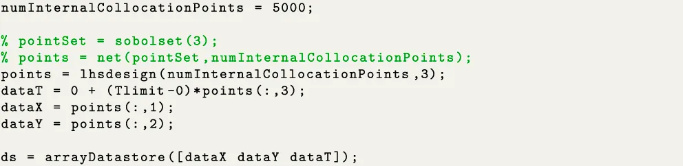
The first part is the input data generation. For the conventional PINNs, points have to be generated 1) in the interior of domain to satisfy the PDE residual, 2) on the boundary of domain to satisfy the boundary conditions, and 3) additional points to satisfy the initial conditions. However, in the modified approach, since the output is adapted so as to satisfy all of the conditions simultaneously, only the interior points are required to be generated. The part of the code generating the interior data points by Latin hypercube sampling has been illustrated in the following snippet.

Initialization of Network Parameters

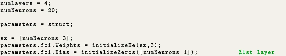
Next, the fully connected deep neural net architecture is constructed according to the user-defined number of layers “numLayers” and number of neurons per layer “numNeurons.” The trainable parameters (weights and biases) for every layer is initialized and stored in the fields of a structure array called “parameters.” The instance of initializing the weights and biases of the first fully connected layer has been captured by the following snippet. Here, the network weights are initialized by the He initialization [17] implemented by the function “initializeHe.” The He initializer samples the weights out of a normal distribution with zero mean and variance $=\frac{2}{N_i}$, where $N_i$ is the number of input channels. This function “initializeHe” takes in two input arguments, one is the size of trainable parameters “sz”and the other is “$N_i$” and returns the sampled weights as a “dlarray” object. Note that “dlarray” is a built-in deep learning array in MATLAB employed for customizing the training process of DNNs. It enables numerous numerical operations including the computation of derivatives through AD. The network biases have been initialized by the zeros initialization implemented by the function “initializeZeros.” As it is evident that the initialization schemes can be easily customized, other initializers like Glorot or Xavier, Gaussian, orthogonal and others can be readily employed depending on the model type and choice of the user. In fact, a wide variety of initialization schemes of trainable parameters for various type of DNNs can be found in the MATLAB documentation.¹

Neural Network Training

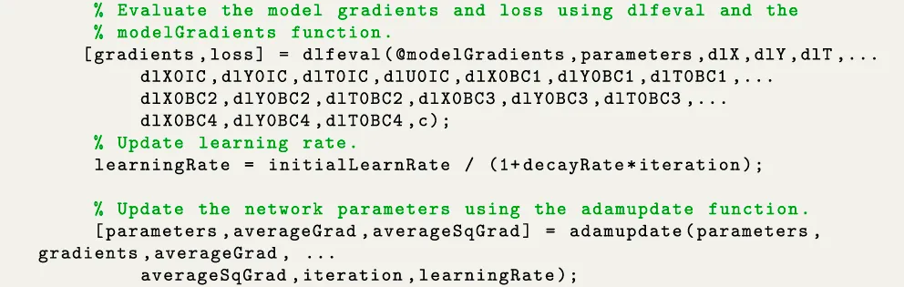
At this stage, the network is to be trained with user-specified value of parameters like, number of epochs, initial learning, decay rate along with several other tuning options. It is worth noting that multiple facilities to allocate hardware resources are available in MATLAB for training the network in an optimal computational cost. This include using CPU, GPU, multi GPU, parallel (local or remote) and cloud computing. The steps performed during the model training within the nested loops of epoch and iteration in mini-batches have been illustrated in the following snippet. To recall, an epoch is the full pass of the training algorithm over the entire training set and an iteration is one step of the gradient descent algorithm towards minimizing the loss function using a mini-batch. As it can be observed from the snippet that three operations are involved during the model training. These are 1) evaluating the model gradients and loss using “dlfeval”² by calling the function “modelGradients” (which is explained in the next snippet), 2) updating the learning rate with every iteration and epoch and 3) finally updating the network parameters during the backpropagation using adaptive moment estimation (ADAM) [18]. In addition to ADAM, other stochastic gradient descent algorithms like, stochastic gradient descent with momentum (SGDM) and root mean square propagation (RMSProp) can be readily implemented via their built-in MATLAB routines.

Encoding the Physics in the Loss Function

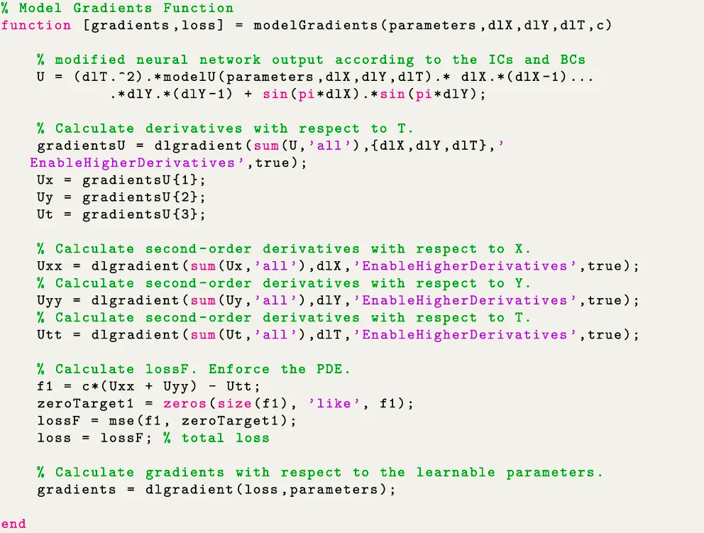
The next snippet presents the function “modelGradients.” This sub-routine is the distinctive feature of PINNs where the physics of the problem is encoded in the loss functions. As mentioned previously, in conventional PINNs, the system response is assumed to be a DNN such that U=modelU(parameters,dlX,dlY,dlT). A difference to the expression of U can be observed in this snippet where the DNN output is modified based on the ICs and BCs. As obvious, this modification will change from problem to problem. In this case, the expression is shown for illustration and is related to Eq. 33 of Example 4 defined in the next section. As the name “dlgradient” suggests, it is used to compute the derivatives via AD. After evaluating the gradients, the loss term enforcing the PDE residual is computed.

As the modified DNN output ensures the satisfaction of ICs and BCs, only the loss term corresponding to PDE residual is necessary. Instead, if conventional PINNs was used, separate loss terms originating from the ICs and BCs would have to be added to the residual loss. Finally, the gradients of the combined loss w.r.t. the network parameters are computed and passed as the function output. These gradients are further used during backpropagation.

As obvious, there will be another loss term involved while solving an inverse problem which minimizes the discrepancy between the model prediction and the measured data. The parameter to be identified is updated as another additional hyperparameter of the DNN along with the network weights and biases. This can be easily implemented by adding the following line: c_update = parameters.(“fc” + numLayers).opt_param; and evaluating the PDE residual as f1 = c_update*(Uxx + Uyy) - Utt in Example 4. In doing so, note that c in line 22 of the snippet will be replaced by c_update.

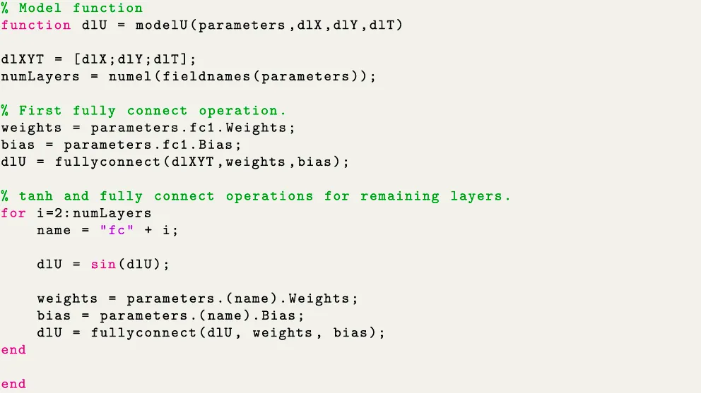
Fully Connect Operations

The “modelU” function has been illustrated in the next snippet. Here, the fully connected deep neural network (FC-DNN) model is constructed as per the dimensionality of input and network parameters. In particular, the fully connect operations are performed via “fullyconnect.” This function uses the weighted sum to connect all the inputs to each output feature using the “weights,” and adds a “bias.” Sinusoidal activation function has been used here. The sub-routine returns the weighted output features as a dlarray “dlU” having the same underlying data type as the input “dlXYT.”

Once the PINNs model is trained, it can be used to predict on the test dataset. It is worth noting that the deep learning library of MATLAB is rich and consists of a diverse range of built-in functions, providing the users adequate choice and modelling freedom. In the next section, the performance of conventional and modified PINNs is accessed for solving four representative structural vibration problems, involving solution of ODE including multi-DOF systems, and PDE. In doing so, both forward and inverse problems have been addressed. Complete executable MATLAB codes of PINNs implementation for all the example problems can be found in the Supplementary Material.

Numerical Examples

Forced Vibration of an Undamped Spring-Mass System

The forced vibration of the spring-mass system can be expressed by

$\ddot{u}+{\omega }_n^{2}u=f_0\sin \omega t(12)$

where u, ü, ω_n, f_n, ω and t represent displacement, acceleration, natural frequency, forcing amplitude, forcing frequency and time, respectively. The initial conditions are u(t = 0) = 0 and ü (t = 0) = 0, where ü represents the velocity. The analytical solution to the above system is given by

$u\left(t\right)=\frac{f_0}{{\omega }_n^2-{\omega }^2}\left(\sin \omega t-r\sin {\omega }_{n}t\right)(13)$

where, r = ω/ω_n is the frequency ratio.

As mentioned previously, in the realm of the PINNs framework, solution space (of the ODE, for this case) can be approximated by DNN such that $\widehat{u}={\mathcal{N}}_u(t,\mathit{\theta })$, where the residual of ODE is evaluated with the help of AD. Essentially, this is an optimization problem which can be expressed as,

$\underset{\mathit{\theta }\in {\mathbb{R}}^d}{\mathrm{arg\; min}}\mathcal{L}\left(\mathit{\theta }\right)≔{\left|\left|\frac{{\partial }^2\widehat{u}}{\partial t^2}+{\omega }_n^2\widehat{u}-f_0\sin \omega t\right|\right|}_2+{\left|\left|\widehat{u}\left(t=0\right)\right|\right|}_2+{\left|\left|\frac{\partial \widehat{u}}{\partial t}\left(t=0\right)\right|\right|}_2(14)$

where, $\Vert ◦\Vert$ denotes ${\ell }_2$-norm. For the numerical illustration, it is assumed that $\omega =3$, $r=1.5$ and $f_0=1$. The displacement $u$ is approximated using a fully-connected neural network with 4 hidden layers and 20 neurons per layer. Sinusoidal activation function has been used due to the known periodic nature of the data [19]. 20,000 collocation points have been generated for time data $t\in [04\pi ]$ with the help of Latin hypercube sampling. The neural network is run for 1,000 epochs and the mini-batch size is 1,000. The initial learning rate is assumed to be 0.01 and the popular ADAM optimizer is employed. For testing the PINNs framework, 5,000 points were uniformly generated for time $t\in [04\pi ]$. The solution $\widehat{u}$ obtained using the PINNs framework has been compared with the actual (analytical) solution $u$ in Figure 2A.

Figure 2

Figure 2. Results of the forced spring-mass system (A) Forward solution without modifying the neural network output. (B) Forward solution after modifying the neural network output. (C) Inverse solution in the form of convergence of the identified parameter $\omega$.

It can be observed from Figure 2A that the conventional PINNs framework is not capable of capturing the time response variation satisfactorily. As discussed in the previous sections, the reason is related to the regularization of the loss term in Eq. 14 and has been recently addressed in [16]. Although their approach proved to be effective, it entails extra computational effort.

Therefore, an alternative approach has been employed in this work to address the scaling issue which requires no additional computational cost compared to that of conventional PINNs. For avoiding multiple terms in the loss function, a simple scheme for modifying the neural network output has been adopted so that the initial and/or, boundary conditions are satisfied. To automatically satisfy the initial conditions in the above problem, the output of the neural network $\widehat{u}$ is modified as,

${\widehat{u}}_{\text{mod}}=t\widehat{u}(15)$

Since the modified neural network output is ${\widehat{u}}_{\text{mod}}$, the new loss function can be expressed as,

$\underset{\mathit{\theta }\in {\mathbb{R}}^d}{\mathrm{arg\; min}}{\mathcal{L}}_{\text{new}}\left(\mathit{\theta }\right)≔{\left|\left|\frac{{\partial }^2{\widehat{u}}_{\text{mod}}}{\partial t^2}+{\omega }_n^2{\widehat{u}}_{\text{mod}}-f_0\sin \omega t\right|\right|}_2(16)$

Following this approach, significant improvement in approximation of the displacement response has been achieved as shown in Figure 2B. Next, the implementation of PINNs has been illustrated for an inverse setting. For doing so, the same problem as defined by Eq. 12 is re-formulated such that the displacement time history is given in the form of measurements and the natural frequency ${\omega }_n$ has to be identified. The optimization problem can be expressed as,

$\underset{\mathit{\theta }\in {\mathbb{R}}^d,\omega \in \mathbb{R}}{\mathrm{arg\; min}}\mathcal{L}\left(\mathit{\theta },\omega \right)≔{\left|\left|\frac{{\partial }^2\widehat{u}}{\partial t^2}+{\omega }_n^2\widehat{u}-f_0\sin \omega t\right|\right|}_2+{\left|\left|\widehat{u}-u^{*}\right|\right|}_2(17)$

where, $u^{*}$ represents the measured displacement data. 15,000 collocation points have been generated for time data $t\in [04\pi ]$ with the help of Latin hypercube sampling. 2,500 displacement data points were used for artificially simulating the measurement data and 5$\%$ uniform random noise was added. The architecture and the parameters of the neural network is the same as the previous case. The results have been presented in the form of convergence of the identified parameter $\omega$ in Figure 2C. The converged value of $\omega =3.0$ demonstrates exact match with the actual value. It is worth mentioning that the PINNs framework is inherently adapted to also provide the solution to the ODE along with the identified parameter in the inverse setup. This demonstrates that the PINNs framework can be easily adapted for solving forward and inverse problems in structural vibration.

Forced Vibration of a Damped Spring-Mass System

The second example concerns a forced vibration of a damped spring-mass system and can be expressed by

$\ddot{u}+2\zeta {\omega }_n\dot{u}+{\omega }_n^{2}u=f_0\sin \omega t(18)$

where u, $\dot{u}$, ü, ω_n, ζ, f₀, ω and t represent displacement, velocity, acceleration, natural frequency, damping ratio, forcing amplitude, forcing frequency and time, respectively. The initial conditions are u(t = 0) = 0 and $\dot{u}$(t = 0) = 0. The analytical solution to the above system can be found in [20].

As mentioned previously, in the realm of the PINNs framework, solution space (of the ODE, for this case) can be approximated by DNN such that $\widehat{u}={\mathcal{N}}_u(t,\mathit{\theta })$, where the residual of ODE is evaluated with the help of AD. Essentially, this is an optimization problem which can be expressed as,

$\underset{\mathit{\theta }\in {\mathbb{R}}^d}{\mathrm{arg\; min}}\mathcal{L}\left(\mathit{\theta }\right)≔{\left|\left|\frac{{\partial }^2\widehat{u}}{\partial t^2}+2\zeta {\omega }_n\frac{\partial \widehat{u}}{\partial t}+{\omega }_n^2\widehat{u}-f_0\sin \omega t\right|\right|}_2+{\left|\left|\widehat{u}\left(t=0\right)\right|\right|}_2+{\left|\left|\frac{\partial \widehat{u}}{\partial t}\left(t=0\right)\right|\right|}_2(19)$

where, $\Vert ◦\Vert$ denotes ${\ell }_2$-norm. For the numerical illustration, it is assumed that $\omega =3$, $\zeta =0.025$, $r=1.5$ and $f_0=1$. The displacement $u$ is approximated using a fully-connected neural network with 4 hidden layers and 20 neurons per layer. Sinusoidal activation function has been used due to the known periodic nature of the data [19]. The neural network is run for 1,000 epochs and the mini-batch size is 1,000. The initial learning rate is assumed to be 0.01 and the popular ADAM optimizer is employed. The solution $\widehat{u}$ obtained using the PINNs framework has been compared with the actual (analytical) solution $u$ in Figure 3A. 20,000 collocation points have been generated for time data $t\in [08\pi ]$ with the help of Latin hypercube sampling to obtain the results in Figures 3A, B. For testing the PINNs framework, 5,000 points were uniformly generated for time $t\in [08\pi ]$ to obtain the results in Figures 3A, B.

Figure 3

Figure 3. Results of the damped forced spring-mass system (A) Forward solution without modifying the neural network output. (B) Forward solution after modifying the neural network output. (C) Forward solution over extended time after modifying the neural network output to observe the steady state response (after the transients have died out).

It can be observed from Figure 3A that the conventional PINNs framework is not capable of capturing the time response variation satisfactorily. As discussed in the previous sections, the reason is related to the regularization of the loss term in Eq. 14. Therefore, to automatically satisfy the initial conditions, modified output of the neural network ${\widehat{u}}_{\text{mod}}$ is the same as Eq. 15 as the initial conditions are identical to that of the first example. Therefore, the new loss function can be expressed as,

$\underset{\mathit{\theta }\in {\mathbb{R}}^d}{\mathrm{arg\; min}}{\mathcal{L}}_{\text{new}}\left(\mathit{\theta }\right)≔{\left|\left|\frac{{\partial }^2{\widehat{u}}_{\text{mod}}}{\partial t^2}+2\zeta {\omega }_n\frac{\partial {\widehat{u}}_{\text{mod}}}{\partial t}+{\omega }_n^2{\widehat{u}}_{\text{mod}}-f_0\sin \omega t\right|\right|}_2(20)$

Following this approach, significant improvement in approximation of the displacement response has been achieved as shown in Figure 3B. The displacement response is presented over extended time in Figure 3C so as to investigate the performance of PINNs on the steady state response after the transients have died out. For generating the result in Figure 3C, 60,000 collocation points have been generated for the time data $t\in [050]$ for training the network. For testing the PINNs framework, 40,000 points were uniformly generated for time $t\in [050]$. The approximation by PINNs is found to be excellent in terms of capturing the response trends.

Next, the implementation of PINNs has been illustrated for an inverse setting. For doing so, the same problem as defined by Eq. 18 is re-formulated such that the displacement time history is given in the form of measurements and both natural frequency ${\omega }_n$ and damping ratio $\zeta$ have to be identified simultaneously. The optimization problem can be expressed as,

$\underset{\mathit{\theta }\in {\mathbb{R}}^d,\omega \in \mathbb{R}}{\mathrm{arg\; min}}\mathcal{L}\left(\mathit{\theta },\omega \right)≔{\left|\left|\frac{{\partial }^2\widehat{u}}{\partial t^2}+2\zeta {\omega }_n\frac{\partial \widehat{u}}{\partial t}+{\omega }_n^2\widehat{u}-f_0\sin \omega t\right|\right|}_2+{\left|\left|\widehat{u}-u^{*}\right|\right|}_2(21)$

where, $u^{*}$ represents the measured displacement data. 10,000 collocation points have been generated for time data $t\in [04\pi ]$ with the help of Latin hypercube sampling. 1,000 displacement data points were used for artificially simulating the measurement data and 1$\%$ uniform random noise was added. The architecture and the parameters of the neural network is the same as the previous case.

The results have been presented in the form of convergence of the identified parameters (natural frequency and damping ratio) in Figure 4. The converged value of ${\omega }_n=2.9985$ and $\zeta =0.0097$ demonstrate close match with the actual values of 3 and 0.01, respectively. This demonstrates that the PINNs framework can be easily adapted for solving forward and inverse problems in structural vibration.

Figure 4

Figure 4. Identification results for the damped forced spring-mass system (A) Convergence of the identified natural frequency. (B) Convergence of the identified damping ratio.

Free Vibration of a 2-DOF Discrete System

A 2-DOF lumped mass system as shown in Figure 5 is considered in this example [20]. This example has been included to illustrate the application of PINNs in a multi-output setting for the inference and identification of multi degree of freedom systems. The governing ODE and the initial conditions are as follows,

$\begin{array}{cc}\hfill & \left[\begin{array}{cc}\hfill m_1\hfill & \hfill 0\hfill \\ \hfill 0\hfill & \hfill m_2\hfill \end{array}\right]\left\{\begin{array}{c}\hfill {\ddot{q}}_1\hfill \\ \hfill {\ddot{q}}_2\hfill \end{array}\right\}+\left[\begin{array}{cc}\hfill c_1+c_2\hfill & \hfill -c_2\hfill \\ \hfill -c_2\hfill & \hfill c_2+c_3\hfill \end{array}\right]\left\{\begin{array}{c}\hfill {\dot{q}}_1\hfill \\ \hfill {\dot{q}}_2\hfill \end{array}\right\}\hfill \\ \hfill & +\left[\begin{array}{cc}\hfill k_1+k_2\hfill & \hfill -k_2\hfill \\ \hfill -k_2\hfill & \hfill k_2+k_3\hfill \end{array}\right]\left\{\begin{array}{c}\hfill q_1\hfill \\ \hfill q_2\hfill \end{array}\right\}=\left\{\begin{array}{c}\hfill f_1\hfill \\ \hfill f_2\hfill \end{array}\right\}\hfill \end{array}(22)$

with initial conditions $\mathit{q}(0)$ and $\dot{\mathit{q}}(0)$. In Eq. 22, $q_i$, ${\dot{q}}_i$, ${\ddot{q}}_i$ represent the displacement, velocity, acceleration of the $i^{\text{th}}$ DOF, respectively, $m_i$ and $f_i$ represent the mass of the $i^{\text{th}}$ DOF and force acting at the $i^{\text{th}}$ DOF, respectively, $c_j$ and $k_j$ are the damping and stiffness coefficient of the $j^{\text{th}}$ connecting element, respectively. For this 2-DOF system, $i=\mathrm{1,2}$ and $j=\mathrm{1,2,3}$. Since the free vibration problem has been undertaken, the right hand side of Eq. 22 is zero. Two cases of the free vibration problem have been considered, undamped and damped. For each of these cases, both forward and inverse formulations have been presented. The analytical solution to the above governing ODE considering undamped and damped cases, respectively, can be determined as,

$\mathit{q}\left(t\right)={\displaystyle \sum _{i=1}^n}{d}_i{\mathit{u}}_i\cos \left({\omega }_{i}t-{\varphi }_i\right)(23)$

$\mathit{q}\left(t\right)={\displaystyle \sum _{i=1}^n}{d}_i{\mathit{u}}_i{\mathrm{e}}^{-{\zeta }_i{\omega }_{i}t}\cos \left({\omega }_{di}t-{\varphi }_i\right)(24)$

where, constants $d_i$ and ${\varphi }_i$ have to be determined from the given initial conditions. $n$ represents the number of DOFs, therefore $n=2$ for the above system. ${\omega }_i$ and ${\mathit{u}}_i$ are the $i^{\text{th}}$ undamped natural frequency and mode shape vector, respectively, obtained from the modal analysis. In Eq. 24, ${\zeta }_i$ and ${\omega }_{di}$ represent the $i^{\text{th}}$ damping ratio and damped natural frequency, respectively.

Figure 5

Figure 5. A schematic representation of the 2-DOF lumped mass system.

As opposed to the previous examples, in general, the response associated with each DOF has to be represented by an output node of (multi-output) FC-DNN. Since the above example is a 2-DOF system, the response of the two DOFs are represented by two output nodes of an FC-DNN in the realm of PINNs architecture such that $\widehat{\mathit{q}}=\left\{\begin{array}{c}\hfill {\widehat{q}}_1\hfill \\ \hfill {\widehat{q}}_2\hfill \end{array}\right\}={\mathcal{N}}_q(t,\mathit{\theta })$. The optimization problem can be expressed as,

$\underset{\mathit{\theta }\in {\mathbb{R}}^d}{\mathrm{arg\; min}}\mathcal{L}\left(\mathit{\theta }\right)≔{\left|\left|\mathbf{M}\ddot{\widehat{\mathit{q}}}+\mathbf{C}\dot{\widehat{\mathit{q}}}+\mathbf{K}\widehat{\mathit{q}}\right|\right|}_2+{\left|\left|\widehat{\mathit{q}}\left(t=0\right)-{\mathit{q}}_0\right|\right|}_2+{\left|\left|\dot{\widehat{\mathit{q}}}\left(t=0\right)\right|\right|}_2(25)$

where, the gradients arising in Eq. 25 can be computed by AD. The following parameter values are adopted, $m_1=9$, $m_2=1$, $k_1=24$, $k_2=3$, $k_3=0$, $c_1=1$, $c_2=0.125$, $c_3=0$. An FC-DNN with 4 hidden layers and 20 neurons per layer is used. Sinusoidal activation function has been used due to the known periodic nature of the data. The neural network is run for 1,000 epochs and the mini-batch size is 1,000. The initial learning rate is assumed to be 0.01 and the popular ADAM optimizer is employed. Collocation points have been generated for time data $t\in [08\pi ]$ with the help of Latin hypercube sampling to obtain the results in Figures 6–8. For testing the conventional PINNs framework, 10,000 points were uniformly generated for time $t\in [08\pi ]$ to obtain the results in Figure 6. The undamped and damped time response obtained using conventional PINNs framework have been compared with the actual (analytical) solution in Figure 6.

Figure 6

Figure 6. Results of free vibration of the 2-DOF lumped mass system. (A) Undamped response for IC ${\mathit{q}}_0={\left[\begin{array}{cc}\hfill q_{01}\hfill & \hfill q_{02}\hfill \end{array}\right]}^T={\left[\begin{array}{cc}\hfill 1\hfill & \hfill 3\hfill \end{array}\right]}^T$, ${\dot{\mathit{q}}}_0=\mathbf{0}$. The predicted responses have been obtained using 60,000 collocation points. (B) Undamped response for IC ${\mathit{q}}_0={\left[\begin{array}{cc}\hfill q_{01}\hfill & \hfill q_{02}\hfill \end{array}\right]}^T={\left[\begin{array}{cc}\hfill 1\hfill & \hfill 0\hfill \end{array}\right]}^T$, ${\dot{\mathit{q}}}_0=\mathbf{0}$. The predicted responses have been obtained using 100,000 collocation points. (C) Damped response for IC ${\mathit{q}}_0={\left[\begin{array}{cc}\hfill q_{01}\hfill & \hfill q_{02}\hfill \end{array}\right]}^T={\left[\begin{array}{cc}\hfill 1\hfill & \hfill 3\hfill \end{array}\right]}^T$, ${\dot{\mathit{q}}}_0=\mathbf{0}$. The predicted responses have been obtained using 40,000 collocation points. (D) Damped response for IC ${\mathit{q}}_0={\left[\begin{array}{cc}\hfill q_{01}\hfill & \hfill q_{02}\hfill \end{array}\right]}^T={\left[\begin{array}{cc}\hfill 1\hfill & \hfill 0\hfill \end{array}\right]}^T$, ${\dot{\mathit{q}}}_0=\mathbf{0}$. The predicted responses have been obtained using 120,000 collocation points.

It can be observed from Figure 6 that the conventional PINNs framework is capable of capturing the undamped and damped time response variation satisfactorily for two different ICs. The IC ${\mathit{q}}_0=\left\{\begin{array}{c}\hfill q_{01}\hfill \\ \hfill q_{02}\hfill \end{array}\right\}=\left\{\begin{array}{c}\hfill 1\hfill \\ \hfill 3\hfill \end{array}\right\}$, ${\dot{\mathit{q}}}_0=\mathbf{0}$ is adopted so that the system vibrates with the first natural frequency only as shown in Figures 6A, C, whereas the IC ${\mathit{q}}_0=\left\{\begin{array}{c}\hfill q_{01}\hfill \\ \hfill q_{02}\hfill \end{array}\right\}=\left\{\begin{array}{c}\hfill 1\hfill \\ \hfill 0\hfill \end{array}\right\}$, ${\dot{\mathit{q}}}_0=\mathbf{0}$ is a more general one resulting in a multi-frequency response as shown in Figures 6B, D. It is worth mentioning that the beat phenomenon exists in the free response of the above 2-DOF system due to close proximity of the two natural frequencies (${\omega }_1=\sqrt{2}$ and ${\omega }_2=2$).

Next, PINNs has been implemented in an inverse setup for identification of system parameters both for the undamped and damped cases. For doing so, the same problem as defined by Eq. 22 is re-formulated such that the displacement time history data is available in the form of measurements and stiffness parameters ($k_1$ and $k_2$) for the undamped case and stiffness and damping parameters ($k_1$, $k_2$, $c_1$ and $c_2$) for the damped case, have to be identified simultaneously. The optimization problem for the undamped and damped case, respectively, can be expressed as,

$\underset{\mathit{\theta }\in {\mathbb{R}}^d,k_1,k_2\in \mathbb{R}}{\mathrm{arg\; min}}\mathcal{L}\left(\mathit{\theta },k_1,k_2\right)≔{\left|\left|\mathbf{M}\ddot{\widehat{\mathit{q}}}+\mathbf{K}\widehat{\mathit{q}}\right|\right|}_2+{\left|\left|\widehat{\mathit{q}}-{\mathit{q}}^{*}\right|\right|}_2(26)$

$\underset{\mathit{\theta }\in {\mathbb{R}}^d,k_1,k_2,c_1,c_2\in \mathbb{R}}{\mathrm{arg\; min}}\mathcal{L}\left(\mathit{\theta },k_1,k_2,c_1,c_2\right)≔{\left|\left|\mathbf{M}\ddot{\widehat{\mathit{q}}}+\mathbf{C}\dot{\widehat{\mathit{q}}}+\mathbf{K}\widehat{\mathit{q}}\right|\right|}_2+{\left|\left|\widehat{\mathit{q}}-{\mathit{q}}^{*}\right|\right|}_2(27)$

where, $q^{*}$ represents the measured displacement data. Collocation points have been generated for time data $t\in [08\pi ]$ with the help of Latin hypercube sampling. 2,000 displacement data points were used for artificially simulating the measurement data and 1% uniform random noise was added. The architecture and the parameters of the neural network is the same as the forward formulation. The results have been presented in the form of convergence of identified system parameters in Figures 7, 8 for the undamped and damped case, respectively.

Figure 7

Figure 7. Identification results for the undamped 2-DOF system (A) Convergence of the identified stiffness parameter $k_1$. (B) Convergence of the identified stiffness parameter $k_2$. For obtaining these results, 45,000 collocation points and 2,000 data points with 1% random uniform noise were used to train the PINNs model.

Figure 8

Figure 8. Identification results for the damped 2-DOF system (A) Convergence of the identified stiffness parameter $k_1$, (B) Convergence of the identified stiffness parameter $k_2$, (C) Convergence of the identified damping parameter $c_1$, (D) Convergence of the identified damping parameter $c_2$. For obtaining these results, 70,000 collocation points and 2000 data points with 1% random uniform noise were used to train the PINNs model.

The converged values of $k_1=24.0031$ and $k_2=2.9995$ have been obtained from Figure 7 for the undamped case. The converged values of $k_1=24.0064$, $k_2=2.9995$, $c_1=1.0030$ and $c_2=0.1248$ have been obtained from Figure 8 for the damped case. The converged values of identified system parameters demonstrate close match with the actual values $k_1=24$, $k_2=3$, $c_1=1$ and $c_2=0.125$. This demonstrates that the PINNs framework can be easily adapted for solving forward and inverse problems in multi-DOF systems. In addition to the adopted strategy to employ a single two-output FC-DNN to solve a 2-DOF system, two individual single output FC-DNNs were investigated. However, the latter failed to map the time response accurately due to the inability of two independent networks to adequately capture the dependencies of the coupled differential equations and hence, minimize the loss.

Free Vibration of a Rectangular Membrane

A rectangular membrane with unit dimensions excited by an initial displacement $u=\sin \pi x\sin \pi y$ has been considered in this example. The governing partial differential equation (PDE), initial and boundary conditions can be expressed as

$c{\nabla }^{2}u=c\left(\frac{{\partial }^{2}u}{\partial x^2}+\frac{{\partial }^{2}u}{\partial y^2}\right)=\frac{{\partial }^{2}u}{\partial t^2}\forall x,y\in \left[\mathrm{0,1}\right],t>0(28)$

$u=0\forall x,y\in {\mathrm{\Gamma }}_u(29)$

$u=\sin \pi x\sin \pi y\forall t=0,x,y\in \left[\mathrm{0,1}\right](30)$

$\frac{\partial u}{\partial t}=0\forall t=0,x,y\in \left[\mathrm{0,1}\right](31)$

where, $u$ is the displacement and $c$ is the velocity of wave propagation. In Eqs 28–31, $x$, $y$ represent the spatial coordinates, $t$ represents time and ${\mathrm{\Gamma }}_u$ denotes the spatial domain. The analytical solution to the governing PDE is $u(x,y,t)=\sin \pi x\sin \pi y\cos \sqrt{2}\pi t$.

Using the PINNs framework, solution of the PDE is approximated by a DNN such that $\widehat{u}={\mathcal{N}}_u(x,y,t,\mathit{\theta })$, where residual of the PDE is evaluated with the help of AD. The optimization problem can be expressed as,

$\begin{array}{c}\hfill \underset{\mathit{\theta }\in {\mathbb{R}}^d}{\mathrm{arg\; min}}\mathcal{L}\left(\mathit{\theta }\right)≔{\left|\left|c\left(\frac{{\partial }^2\widehat{u}}{\partial x^2}+\frac{{\partial }^2\widehat{u}}{\partial y^2}\right)-\frac{{\partial }^2\widehat{u}}{\partial t^2}\right|\right|}_2+{\left|\left|\widehat{u}\left(x,y\in {\mathrm{\Gamma }}_u\right)\right|\right|}_2+{\left|\left|\widehat{u}\left(t=0\right)-\sin \pi x\sin \pi y\right|\right|}_2+\\ \hfill {\left|\left|\frac{\partial \widehat{u}}{\partial t}\left(t=0\right)\right|\right|}_2\end{array}(32)$

The displacement $u$ is approximated using a fully-connected neural network with 4 hidden layers and 20 neurons per layer. Sinusoidal activation function has been used. 5,000 collocation points are generated for the spatial $x,y\in [01]$ and temporal data $t\in [01/(2\sqrt{2})]$ with the help of Latin hypercube sampling. The neural network is run for 1,000 epochs and the mini-batch size is 1,000. The initial learning rate is assumed to be 0.01 and the popular ADAM optimizer is employed. For testing the PINNs framework, 1,000 points were uniformly generated for $x,y$ and $t$. The solution in space obtained using the PINNs framework $\widehat{u}$ (Figure 9B) has been compared with the actual (analytical) solution $u$ (Figure 9A) for four different time instants $t=0.1,0.15,0.2$ and 0.25.

Figure 9

Figure 9. Results of free vibration of the rectangular membrane (A) True forward spatial solution, (B) Predicted forward spatial solution by conventional PINNs, (C) Predicted forward spatial solution by modified PINNs, (D) Inverse solution in the form of convergence of the identified parameter $c$.

It can be observed from Figure 9B that the conventional PINNs framework is not capable of capturing the time response variation satisfactorily. The reason is once again related to the regularization of the loss term in Eq. 32. The different terms related to the residual, initial and boundary conditions in the loss function are not satisfied simultaneously. Specifically, the fact that the condition $u=0$ at the boundary of the domain not being satisfied in the predicted response by conventional PINNs can be visualized from Figure 9B.

To ensure the satisfaction of residual, initial and boundary conditions and improve upon the approximation accuracy, the neural network output has been modified as,

${\widehat{u}}_{\text{mod}}=t^{2}x\left(x-1\right)y\left(y-1\right)\widehat{u}+\sin \pi x\sin \pi y(33)$

Since the modified neural network output is ${\widehat{u}}_{\text{mod}}$, the new optimization problem can be expressed as,

$\underset{\mathit{\theta }\in {\mathbb{R}}^d}{\mathrm{arg\; min}}{\mathcal{L}}_{\text{new}}\left(\mathit{\theta }\right)≔{\left|\left|c\left(\frac{{\partial }^2{\widehat{u}}_{\text{mod}}}{\partial x^2}+\frac{{\partial }^2{\widehat{u}}_{\text{mod}}}{\partial y^2}\right)-\frac{{\partial }^2{\widehat{u}}_{\text{mod}}}{\partial t^2}\right|\right|}_2(34)$

Following this modified PINNs approach, significant improvement in the spatial distribution of the displacement response has been achieved as shown in Figure 9C. Next, the implementation of PINNs has been illustrated in solving another inverse problem. For doing so, the same problem as defined by Eqs 28–31 is re-formulated such that the displacement time history is given in the form of measurements and the wave velocity $c$ has to be identified. The optimization problem can be expressed as,

$\underset{\mathit{\theta }\in {\mathbb{R}}^d,c\in \mathbb{R}}{\mathrm{arg\; min}}\mathcal{L}\left(\mathit{\theta },c\right)≔{\left|\left|c\left(\frac{{\partial }^2\widehat{u}}{\partial x^2}+\frac{{\partial }^2\widehat{u}}{\partial y^2}\right)-\frac{{\partial }^2\widehat{u}}{\partial t^2}\right|\right|}_2+{\left|\left|\widehat{u}-u^{*}\right|\right|}_2(35)$

where, $u^{*}$ represents the measured displacement data. 25,000 collocation points have been generated for spatial coordinates $x,y\in [01]$ and time $t\in [01/(2\sqrt{2})]$ with the help of Latin hypercube sampling. 5,000 displacement data points were used for artificially simulating the measurement data and 2$\%$ uniform random noise was added. The architecture and the parameters of the neural network is the same as for the forward problem. The results have been presented in the form of convergence of the identified parameter $c$ at the end of 10,000 epochs in Figure 9D. The converged value of $c=0.9902$ demonstrates good match with the actual value $c=1.0$. It is worth noting that the PINNs framework is inherently adapted to also provide the solution to the PDE along with the identified parameter in the inverse setup. This demonstrates that the PINNs framework can be easily adapted for solving forward and inverse problems in structural vibration.

Summary and Conclusion

This work presents the MATLAB implementation of PINNs for solving forward and inverse problems in structural vibrations. The contribution of the study lies in the following:

1. It is one of the very few applications of PINNs in structural vibrations till date and thus aims to fill-up the gap. This also makes the work timely in nature.

2. It demonstrates a critical drawback of the first generation PINNs while solving vibration problems, which leads to inaccurate predictions.

3. It mostly addresses the above drawback with the help of a simple modification in the PINNs framework without adding any extra computational cost. This results in significant improvement in the approximation accuracy.

4. The implementation of conventional and modified PINNs is performed in MATLAB. As per the authors’ knowledge, this is the first published PINNs code for structural vibrations carried out in MATLAB, which is expected to benefit a wide scientific audience interested in the application of deep learning in computational science and engineering.

5. Complete executable MATLAB codes of all the examples undertaken have been provided along with their line-by-line explanation so that the interested readers can readily implement these codes.

Four representative problems in structural vibrations, involving ODE and PDE have been solved including multi-DOF systems. Both forward and inverse problems have been addressed while solving each of the problems. The results in three examples involving single DOF systems clearly state that the conventional PINNs is incapable of approximating the response due to a regularization issue. The modified PINNs approach addresses the above issue and captures the solution of the ODE/PDE adequately. For the 2-DOF system, the conventional PINNs performs satisfactorily for the inference and identification formulations. It is recommended to employ $n$-output layer neural network to solve $n$-DOF system instead of employing $n$ number of individual neural networks which fails to capture the dependencies of the coupled differential equations (physics).

Making the codes public is a humble and timely attempt for expanding the scientific contribution of deep learning in MATLAB, owing to its recently developed rich deep learning library. The research model can be based similar to that of authors adding their Python codes in public repositories like, GitHub. Since the topic is hot, it is expected to quickly populate with the latest developments and improvements, bringing the best to the research community. The authors can envision a huge prospect of their modest research of a recently developed and widely popular method in a new application field and its implementation in a new and more user-friendly software.

Our investigation of the proposed PINNs approach on complex structural dynamic problems, such as beams, plates, and nonlinear oscillators (e.g., cubic stiffness and Van der Pol oscillator), showed opportunities for improvement. To better capture the forward solution and identify unknown parameters in inverse problems, modifications to the proposed approach in this paper are needed. Based on our observation, the need for further systematic investigation has been identified. This aligns with the recent findings in [21]. Future work should focus on automated weight tuning of fully connected neural networks (e.g., [16]), explore physics-informed neural ODEs [11] and symplectic geometry [22].

Data Availability Statement

The original contributions presented in the study are included in the article/Supplementary Material, further inquiries can be directed to the corresponding author.

Author Contributions

TC came up with the idea of the work, carried out the analysis and wrote the manuscript. MF, SA, and HK participated in weekly brainstorming sessions, reviewed the results and manuscript. MF secured funding for the work. All authors contributed to the article and approved the submitted version.

Funding

The authors declare that financial support was received for the research, authorship, and/or publication of this article. TC gratefully acknowledges the support of the University of Surrey through the award of a faculty start-up grant. All authors gratefully acknowledge the support of the Engineering and Physical Sciences Research Council through the award of a Programme Grant “Digital Twins for Improved Dynamic Design,” grant number EP/R006768.

Conflict of Interest

The authors declare that the research was conducted in the absence of any commercial or financial relationships that could be construed as a potential conflict of interest.

Supplementary Material

The Supplementary Material for this article can be found online at: https://www.frontierspartnerships.org/articles/10.3389/arc.2024.13194/full#supplementary-material

Footnotes

¹https://uk.mathworks.com/help/deeplearning/ug/initialize-learnable-parameters-for-custom-training-loop.html#mw_f7c2db63-96b5-4a81-813e-ee621c9658ce

²Functions passed to ‘dlfeval’are allowed to contain calls to ‘dlgradient’, which compute gradients by using automatic differentiation.

References

1. Baydin, AG, Pearlmutter, BA, Radul, AA, and Siskind, JM. Automatic Differentiation in Machine Learning: A Survey. J Machine Learn Res (2017) 18(1):5595–637.

Google Scholar

2. Abadi, M, Agarwal, A, Barham, P, Brevdo, E, Chen, Z, Citro, C, et al. TensorFlow: Large-Scale Machine Learning on Heterogeneous Distributed Systems. Software (2016). arXiv preprint: 1603.04467. arxiv.org/abs/1603.04467. Available from: http://tensorflow.org/.

Google Scholar

3. Paszke, A, Gross, S, Massa, F, Lerer, A, Bradbury, J, Chanan, G, et al. Pytorch: An Imperative Style, High-Performance Deep Learning Library. In: Advances in Neural Information Processing Systems 32: Annual Conference on Neural Information Processing Systems 2019; December 8–14, 2019; Vancouver, BC. NeurIPS (2019). p. 8024–35.

Google Scholar

4. Chollet, F. Deep Learning With Python. 1st edn. United States: Manning Publications Co. (2017).

5. Lagaris, I, Likas, A, and Fotiadis, D. Artificial Neural Networks for Solving Ordinary and Partial Differential Equations. IEEE Trans Neural Networks (1998) 9(5):987–1000. doi:10.1109/72.712178

PubMed Abstract | CrossRef Full Text | Google Scholar

6. Raissi, M, Perdikaris, P, and Karniadakis, G. Physics-Informed Neural Networks: A Deep Learning Framework for Solving Forward and Inverse Problems Involving Non-Linear Partial Differential Equations. J Comput Phys (2019) 378:686–707. doi:10.1016/j.jcp.2018.10.045

CrossRef Full Text | Google Scholar

7. Karniadakis, GE, Kevrekidis, IG, Lu, L, Perdikaris, P, Wang, S, and Yang, L. Physics-Informed Machine Learning. Nat Rev Phys (2021) 3(6):422–40. doi:10.1038/s42254-021-00314-5

CrossRef Full Text | Google Scholar

8. Xu, Y, Kohtz, S, Boakye, J, Gardoni, P, and Wang, P. Physics-Informed Machine Learning for Reliability and Systems Safety Applications: State of the Art and Challenges. Reliability Eng Syst Saf (2023) 230:108900. doi:10.1016/j.ress.2022.108900

CrossRef Full Text | Google Scholar

9. Li, H, Zhang, Z, Li, T, and Si, X. A Review on Physics-Informed Data-Driven Remaining Useful Life Prediction: Challenges and Opportunities. Mech Syst Signal Process (2024) 209:111120. doi:10.1016/j.ymssp.2024.111120

CrossRef Full Text | Google Scholar

10. Zhang, R, Liu, Y, and Sun, H. Physics-Guided Convolutional Neural Network (Phycnn) for Data-Driven Seismic Response Modeling. Eng Structures (2020) 215:110704. doi:10.1016/j.engstruct.2020.110704

CrossRef Full Text | Google Scholar

11. Lai, Z, Mylonas, C, Nagarajaiah, S, and Chatzi, E. Structural Identification With Physics-Informed Neural Ordinary Differential Equations. J Sound Vibration (2021) 508:116196. doi:10.1016/j.jsv.2021.116196

CrossRef Full Text | Google Scholar

12. Yucesan, YA, Viana, FA, Manin, L, and Mahfoud, J. Adjusting a Torsional Vibration Damper Model With Physics-Informed Neural Networks. Mech Syst Signal Process (2021) 154:107552. doi:10.1016/j.ymssp.2020.107552

CrossRef Full Text | Google Scholar

13. Hu, Y, Guo, W, Long, Y, Li, S, and Xu, Z. Physics-Informed Deep Neural Networks for Simulating S-Shaped Steel Dampers. Comput and Structures (2022) 267:106798. doi:10.1016/j.compstruc.2022.106798

CrossRef Full Text | Google Scholar

14. Deng, W, Nguyen, KT, Medjaher, K, Gogu, C, and Morio, J. Rotor Dynamics Informed Deep Learning for Detection, Identification, and Localization of Shaft Crack and Unbalance Defects. Adv Eng Inform (2023) 58:102128. doi:10.1016/j.aei.2023.102128

CrossRef Full Text | Google Scholar

15. Zhang, M, Guo, T, Zhang, G, Liu, Z, and Xu, W. Physics-Informed Deep Learning for Structural Vibration Identification and Its Application on a Benchmark Structure. Philos Trans R Soc A (2024) 382(2264):20220400. doi:10.1098/rsta.2022.0400

CrossRef Full Text | Google Scholar

16. Wang, S, Teng, Y, and Perdikaris, P. Understanding and Mitigating Gradient Flow Pathologies in Physics-Informed Neural Networks. SIAM J Scientific Comput (2021) 43(5):3055–81. doi:10.1137/20m1318043

CrossRef Full Text | Google Scholar

17. He, K, Zhang, X, Ren, S, and Sun, J. Delving Deep Into Rectifiers: Surpassing Human-Level Performance on Imagenet Classification. arXiv (2015) 1026–34. CoRR abs/1502.01852. doi:10.1109/ICCV.2015.123

CrossRef Full Text | Google Scholar

18. Kingma, DP, and Ba, J. Adam: A Method for Stochastic Optimization. In: 3rd International Conference on Learning Representations, ICLR 2015; May 7–9, 2015; San Diego, CA (2015). Conference Track Proceedings.

Google Scholar

19. Haghighat, E, Bekar, AC, Madenci, E, and Juanes, R. Deep Learning for Solution and Inversion of Structural Mechanics and Vibrations (2021). arXiv:2105.09477.

Google Scholar

20. Inman, D. Engineering Vibrations. 3rd edn. Upper Saddle River, New Jersey: Pearson Education, Inc. (2008).

Google Scholar

21. Baty, H, and Baty, L. Solving Differential Equations Using Physics Informed Deep Learning: A Hand-On Tutorial With Benchmark Tests (2023). Available from: https://hal.science/hal-04002928v2,hal-04002928v2 (Accessed April 18, 2023).

Google Scholar

22. Zhong, Y, Dey, B, and Chakraborty, A. Symplectic Ode-Net: Learning Hamiltonian Dynamics With Control. In: Proc. of the 8th International Conference on Learning Representations (ICLR 2020); April 26–30, 2020; Ethiopia.

Google Scholar