Abstract
Flow field prediction is crucial for evaluating the performance of airfoils and aerodynamic optimization. Computational fluid dynamics (CFD) methods usually require a considerable amount of computational resources and time. In this study, a composite model based on deep learning is proposed for flow field prediction. The variational autoencoder (VAE) model is designed to extract representative features of flow fields. The VAE model is trained to determine the optimal latent variable dimension and Kullback-Leibler (KL) divergence weight. Several physical constraints based on mass conservation and pressure coefficient are introduced to reduce the reconstruction loss and improve the model generalization ability. A DeepONet-MLP model, which combines a deep operator network (DeepONet) and a multilayer perceptron (MLP), is trained to achieve the nonlinear mapping from airfoil shapes and lift coefficients to latent variables in the VAE with fewer parameters. Eventually, a DeepONet-MLP-VAE model, which connects the decoder in VAE with DeepONet-MLP, is applied for fast flow field prediction. The results show that the proposed model can accurately and efficiently predict the transonic flow field, with a mean absolute error of 0.0016 and an average processing time of 0.010 s per flow field, which significantly accelerates the CFD evaluation process.
Introduction
Flow field prediction is crucial in various engineering and scientific applications, such as aerodynamic design [1, 2], automotive engineering [3, 4], meteorology [5], energy [6–9] and environmental science [10]. Therefore, flow field prediction is important for improving the efficiency and accuracy of engineering design. In the field of aerodynamics, accurate and quick prediction of the aerodynamic performance of aircraft has become a crucial research direction. With the continuous advancement of aircraft design, particularly owing to the increasing demand for large civil aircraft, the study of aerodynamic characteristics has become increasingly complex and significant. Supercritical airfoils are widely used in the design of modern civil aircraft [11]. In transonic flow fields, the region around a supercritical airfoil exhibits several typical physical phenomena, such as shock waves, shock/boundary layer interactions, and boundary layer separation [12]. These phenomena significantly influence the transonic cruise efficiency of supercritical airfoils. Hence, effectively obtaining the flow field around an airfoil is important for aerodynamic optimization.
Traditional methods for flow field analysis include experimental tests and numerical simulations. The experimental method involves directly observing and measuring flow parameters through wind tunnel tests [13]. Numerical simulations usually solve a system of equations via computational fluid dynamics (CFD) to obtain the values of flow parameters. The experimental method usually incurs high equipment costs, and the numerical simulation method involves large-scale computations and is time-consuming. Neither method can be effectively applied to rapid decision-making and real-time control in aerodynamic design. Therefore, developing an efficient and accurate method for flow field prediction is essential.
The rise of machine learning (ML) has provided new approaches for flow field prediction. Researchers have proposed various surrogate models, such as Kriging models [14], support vector machines (SVMs) [15], and neural networks (NNs) [16]. The internal parameters of the model are continuously adjusted during the learning process to achieve the optimal prediction results. Leifsson et al. [17] utilized Kriging interpolation with CFD simulation data to establish an auxiliary surrogate model for multi-objective aerodynamic optimization of airfoil shapes. However, surrogate models usually encounter difficulties when they are applied to entire flow field predictions due to their limited depth in capturing intricate flow phenomena.
In recent years, the advancement of deep neural networks (DNNs) has been significantly propelled by various market applications, such as image recognition, natural language processing, and autonomous driving. Renganathan et al. [18] proposed several surrogate models, such as DNN, DNN-GP, and DNN-BO, and incorporated constraints for aerodynamic optimization. Brahmachary et al. [19] utilized proper orthogonal decomposition (POD) as a reduced-order model and employed regression models based on moving least squares and multilayer perceptrons (MLPs) to swiftly and accurately predict the internal flow fields of engine inlets. Raissi et al. [20] used the physics-informed neural network (PINN) to couple the incompressible Navier-Stokes equations with dynamic equations, enabling the prediction of lift and drag forces in vortex-induced vibrations. Wu et al. [21] proposed the ffsGAN model, which is based on generative adversarial networks (GANs), to predict the transonic flow field of supercritical airfoils. Du et al. [22] combined a GAN, an MLP and recurrent neural networks (RNNs) to predict the wing pressure distribution and various force coefficients.
The maturity of DNNs has significantly extended the representational capacity of artificial neural networks (ANNs), enabling them to address more complex fluid dynamics problems. Lu et al. [23] extended the universal approximation theorem to a DNN and proposed a deep operator network (DeepONet) with a small generalization error. Based on the autoencoder (AE) proposed by Rumelhart et al. [24], Kingma et al. [25] further introduced the concept of the variational autoencoder (VAE), which uses probability to represent the latent variable space, thereby improving the stability of the generated results and the model generalization ability. Li et al. [26] incorporated DeepONet into the VAE decoder and constructed a generative model with a grid-based encoder, which was successfully applied to the inverse design of supercritical airfoils.
In the field of computer vision (CV), Sohn et al. [27] introduced convolutional neural networks (CNNs) to enhance the image generation capabilities of VAEs. He et al. [28] proposed the deep residual network (ResNet), which addresses the problems of vanishing gradients and exploding gradients during the training of DNNs, as well as network degradation. With the rapid development of CV, the application of surrogate models in flow field prediction and aerodynamic optimization has gained increasing attention from researchers. Deng et al. [29] utilized convolutional autoencoders (CAEs) as flow field feature extractors and MLPs to analyze the mapping relationship between variables, achieving aerodynamic optimization. Sekar et al. [30] utilized CNN to extract geometric parameters from wing shapes and then employed an MLP model to predict the incompressible laminar flow field around the wing based on the extracted geometric parameters, Reynolds number, and angle of attack. Wang et al. [31] acquired the optimal dimensions of the neural network via principal component analysis (PCA) and developed a generative model based on VAE. The model successfully predicted the 2D pressure and velocity profiles around supercritical airfoils. Dubois et al. [32] used linear variational autoencoders (LVAEs) and VAEs to reconstruct and predict unsteady flow fields, specifically targeting 2D vortex shedding, 2D spatial mixing layers and 3D vortex shedding. Li et al. [33] proposed the physically interpretable variational autoencoder (PIVAE) model by incorporating physical features into the latent variables. The model successfully reconstructed the Mach number distribution along the wall of a supercritical airfoil and was applied to the inverse design of supercritical airfoils. Yang et al. [34] proposed the prior variational autoencoder (PVAE) model, which uses the cruise flow field as a prior reference for the off-design condition prediction. Physical constraints such as mass conservation and aerodynamic coefficients reduce prediction errors and enhance the model generalization ability. Chen et al. [35] proposed the FlowDNN model with mass conservation and the incompressible Navier-Stokes equations as physical constraints for rapid prediction of 2D incompressible flow fields around airfoils. Duru et al. [36] proposed a model based on CNN for predicting airfoil flow fields at high angles of attack. Tan et al. [37] proposed an MLP-VAE hybrid model with good generalization ability. The model can accurately predict flow fields for inlet geometries outside the training dataset. Liu et al. [38] proposed a composite model that combines an ANN and a VAE, which can effectively and accurately reconstruct and predict 3D real-time flow fields.
Despite the widespread success of DNN and CV technologies in providing high-fidelity predictive results for various flow fields, most models were trained only from the data-fitting perspective, which does not consider the impact of physical information. There have been few attempts to accurately predict complex transonic flow fields, which include shock waves and flow separation. Unlike traditional neural networks that learn mappings from vectors to vectors, DeepONet specializes in learning mappings from entire functions (or continuous data) to other functions, which makes it applicable to a wide range of problems in physics, engineering, and applied mathematics. However, the use of DeepONet in current surrogate models for predicting airfoil flow fields is relatively infrequent. In this study, a composite model based on deep learning approach is employed to predict the transonic flow fields of supercritical airfoils. Physical constraints based on mass conservation and local physical constraints of pressure coefficient are introduced into the model training process. The impact of these physical constraints on reconstruction loss is studied in this paper. In addition, a DeepONet-MLP combined model is developed. Compared with the simple MLP structure, the DeepONet-MLP model can achieve the nonlinear mapping from airfoil shapes and lift coefficients to latent variables with fewer parameters.
The details of this paper are organized as follows: Introduction introduces the research background. Data Preparation briefly introduces the dataset and the class shape transformation (CST) method. Machine Learning Framework and Training Implementation presents the structure of the models and the specific forms of the physical constraints. The optimal parameters for the designed networks and the impact of physical constraints are also given. In Flow Field Prediction Results, the predictive results of the proposed network are presented. Conclusion summarizes the study and provides an outlook on future research.
Data Preparation
Airfoil Geometry Description
The CST method [39, 40] can ensure the smoothness of an airfoil shape with relatively few parameters. It is defined by a class function C and a shape function S, as shown in Equation 1.where , , , is the trailing edge thickness and c is the chord length.
The class function C is defined as Equation 2. The values of and are set to 0.5 and 1, respectively, for a supercritical airfoil.
The shape function S is defined by Bernstein polynomials Si, as shown in Equation 3, where represents the undetermined CST parameters and n refers to the order of the Bernstein polynomials.
The Bernstein polynomials are defined by Equation 4. Ki is the binomial coefficient, as shown in Equation 5.
In this study, 6th-order Bernstein polynomials serve as shape functions for the upper and lower surfaces of the airfoil, which has totally 14 parameters to describe the geometric shape of the supercritical airfoil. Figure 1 shows the effectiveness of the CST method in fitting OAT15A. The CST method can efficiently and accurately reconstruct complex airfoil shapes with relatively few parameters. As noted in the legend, ‘real’ represents the real shape of the airfoil and is depicted with a red solid line; ‘fit’ represents the airfoil shape fitted by the CST method and is depicted with a blue dashed line. The maximum error of fitting the OAT15A airfoil is 4.10 × 10⁻⁹c.
FIGURE 1
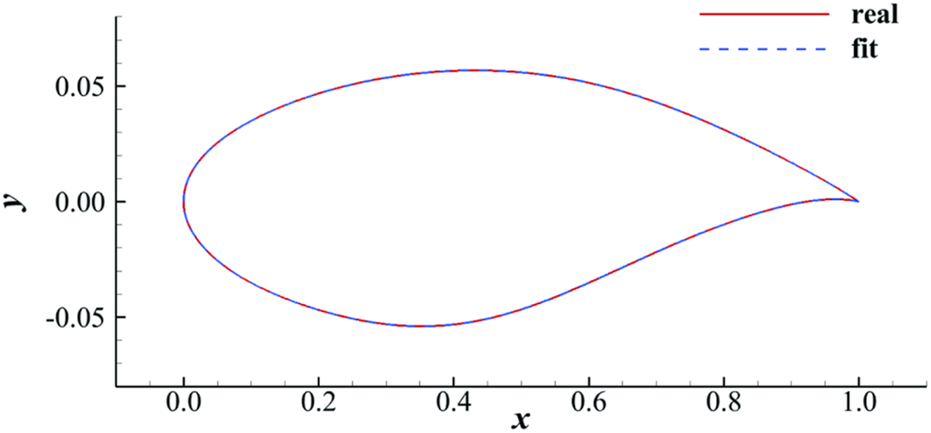
OAT15A fitted by 14 CST parameters.
Transonic Flow Field Dataset of Supercritical Airfoils
The dataset used in this study is a publicly available dataset [34] of supercritical airfoils. The operating conditions of the airfoils are defined by the free stream Mach number Ma, the Reynolds number Re, and the lift coefficient . In this study, the Mach number and Reynolds number are fixed to 0.76 and , respectively, which are typical flow conditions of supercritical airfoil design.
The maximum relative thickness of all airfoils in the dataset is 0.095, which is the case for a wide-body aircraft. An output space sampling (OSS) method [41] was used to sample within the geometric parameter space. A total of 1,498 supercritical airfoil samples are included in the dataset. The geometric shapes of the airfoils and their corresponding pressure coefficient curves are shown in Figure 2.
FIGURE 2
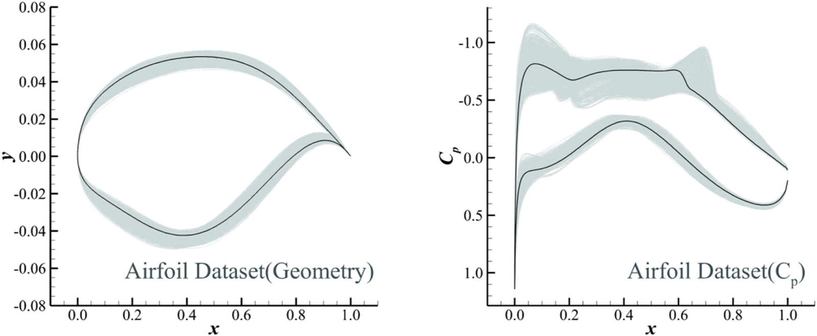
Supercritical airfoils (left) and pressure coefficient (right) curves in the dataset.
CFD Method
A structured C-type grid of the airfoil is automatically generated by an in-house code. The detailed grid generation method is presented in Ref. [42]. The grid structure, which is shown in Figure 3, has 381 points in the circumferential direction and 81 points in the wall-normal direction, with 301 grid points on the airfoil surface. The far-field boundary is located 80 c from the airfoil. The thickness of the first layer of the grid is c to satisfy the requirements of Δy+<1.
FIGURE 3
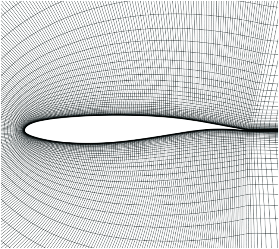
Structured C-type grid of OAT15A.
The flow fields are calculated via the Reynolds-Averaged Navier-Stokes solver CFL3D [43]. The shear stress transport (SST) model is employed for turbulence modeling. The MUSCL scheme, Roe’s scheme, and Gauss-Seidel method are applied for flow variable reconstruction, spatial discretization, and time advancement, respectively. The pressure coefficient Cp distributions of the OAT15A airfoil are computed with different grid sizes and compared with the experimental results [44], as shown in Figure 4. The total number of grid points for the coarse, medium and fine meshes are 15,333, 30,861, and 61,133, respectively. The grid convergence is achieved in the present case. In the following study, the medium grid is applied to dataset generation and machine learning study.
FIGURE 4
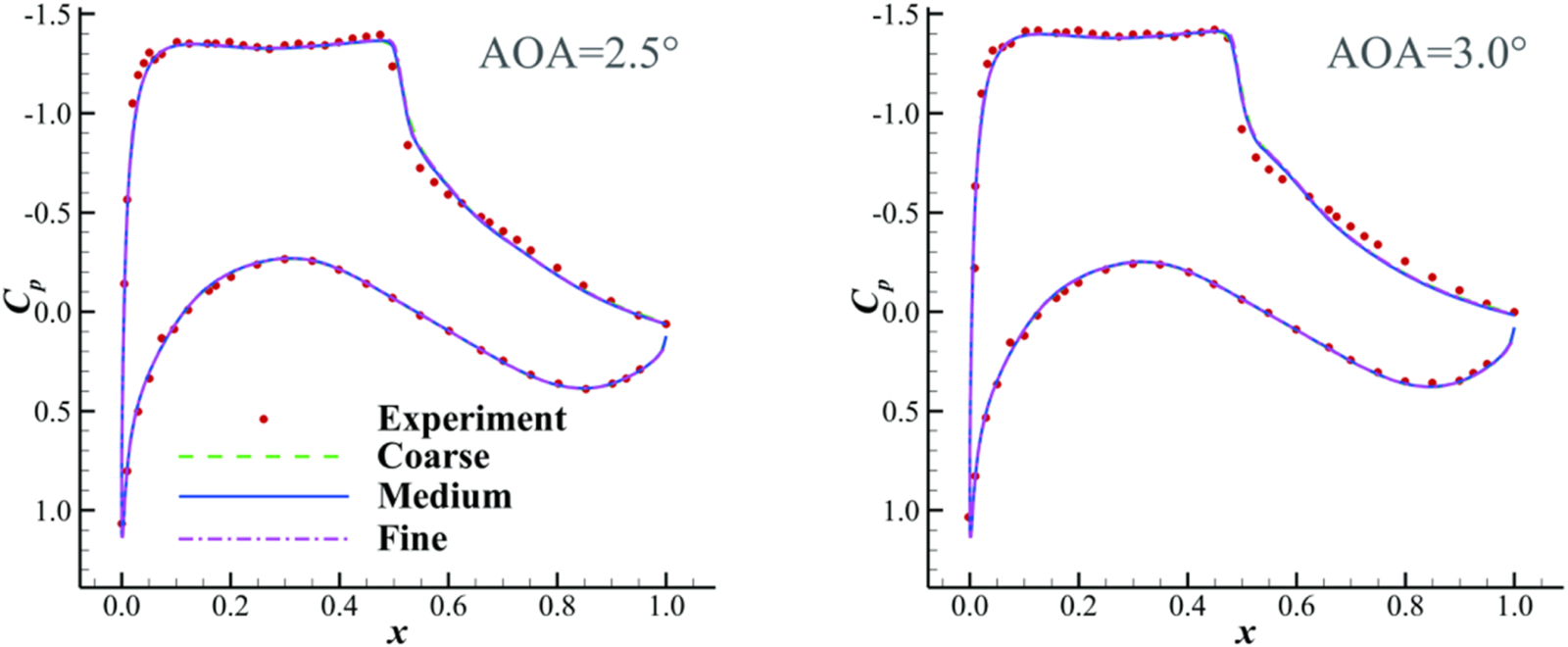
Pressure coefficient distributions of the OAT15A airfoil at Ma = 0.73, Re = 3.0 × 10⁶, and AOA = 2.5 deg (left) and Ma = 0.73, Re = 3.0 × 10⁶, and AOA = 3.0 deg (right).
11 lift coefficients from 0.60 to 1.00 are calculated via CFD for each airfoil in the dataset. All the cases are computed via a fixed lift coefficient CFD method, where the angle of attack is automatically adjusted during CFD iterations to achieve the desired lift coefficient.
In this study, four primary flow variables (pressure p, temperature T, velocity components u and v) are selected to define a single flow field for a 2D airfoil. The grid dimension for numerical computation is 381 × 81. Since the flow field near the airfoil is more critical than the far-field and wake regions, a part of the flow field near the airfoil is extracted from the CFD result for machine learning study, which has 331 × 75 grid points. Each grid point (i, j) can be considered as a pixel of the flow field. Therefore, the flow field plot is reshaped into a matrix of 4 × 331 × 75 floating-point numbers by being unfolded along the circumferential direction (i direction) and the wall-normal direction (j direction), as shown in Figure 5.
FIGURE 5

Transforming a CFD result into a matrix shape.
The dataset contains 1,498 samples of supercritical airfoils. Each sample corresponds to 11 lift coefficients, resulting in a total of 16,478 flow fields. The dataset is divided into three parts: the training set, the validation set and the test set, as shown in Figure 6. 81% of the flow fields are used as the training set. The hyperparameters are adjusted based on the performance on the validation set, which contains 9% of the samples. Finally, 10% of the dataset is used as the test set to evaluate the model’s final predictive performance.
FIGURE 6

Sketch of the dataset splitting and training process.
Normalization is essential because each flow variable has its own range of values and may differ significantly from other variables. Normalizing the input data maps feature ranges to a similar scale, which helps accelerate the convergence speed when training the model. However, normalizing using all training data might fail due to the presence of outliers. Therefore, the flow field is nondimensionalized by the freestream pressure , temperature , velocity components and , as shown in Equation 6.
Machine Learning Framework and Training Implementation
In this study, a DeepONet-MLP-VAE composite model is proposed to realize fast reconstruction and prediction of flow fields. A diagrammatic sketch of the model and its training process is shown in Figure 7. The VAE model is trained to extract features of the flow fields and to realize 2D physical field reconstruction. The DeepONet-MLP is employed to achieve the mapping from the airfoil shapes and lift coefficients to the extracted features. First, the VAE model is trained to determine the optimal latent variable dimension and Kullback-Leibler (KL) divergence weight. Physical constraints based on mass conservation and local constraints of pressure coefficient are introduced in the loss function. Second, a structure combining DeepONet and MLP is designed for the nonlinear mapping from geometric CST parameters and lift coefficients to latent variables of the VAE. Finally, the composite model DeepONet-MLP-VAE is obtained by connecting the DeepONet-MLP with the decoder of the VAE, which can predict the transonic flow fields of supercritical airfoils from geometry parameters and lift coefficients.
FIGURE 7
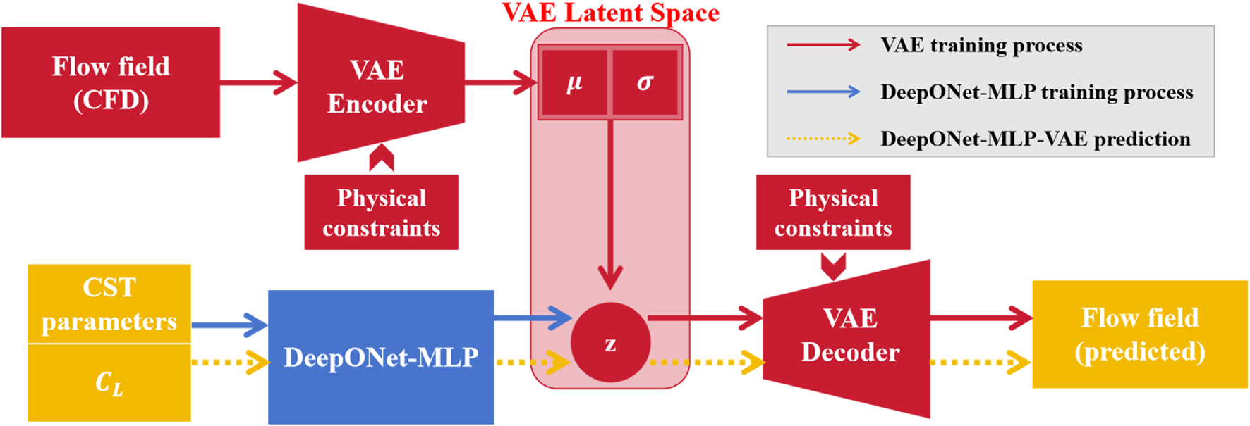
Sketch of the DeepONet-MLP-VAE model framework.
Feature Extraction Model
Flow Field Reconstruction Based on VAE Model
Unsupervised learning is a paradigm of machine learning characterized by the absence of explicit labels or target outputs in the training data. Unlike supervised learning, which relies on predefined target values, unsupervised learning focuses on discovering patterns, structures, or regularities within the data itself. It aims to learn the underlying structure of the data without requiring prelabeled targets. The autoencoder (AE) is an unsupervised learning neural network model comprising two main components: an encoder and a decoder. The encoder compresses the input data into a latent space representation, while the decoder reconstructs the original data from this compressed form. This process enables the AE to perform various tasks, such as data compression, denoising, and feature learning, by learning a compact and meaningful representation of the input data. The model learns to capture the essential features of the input by minimizing the reconstruction loss between the original input and its reconstruction.
The encoding mapping is denoted as , and the decoding mapping is denoted as . The principle of the AE is represented by Equations 7, 8, where q is the input, z is the latent variable and is the output. The training process involves fitting and to minimize the difference between q and .
The variational principle [45] has been introduced based on AE, which is referred to as VAE. Compared with traditional AE, VAE is easier to implement and offers a more stable training process. The encoder’s output of VAE connects to two fully connected layers to derive the mean value and standard deviation . The latent variables are sampled from a normal distribution defined by and . The primary advantage of VAE is the ability to control the distribution of latent variables.
In this study, the input of the VAE consists of six-channel flow field data. These channels include the C-type grid coordinates x and y, pressure p, temperature T, and velocity components u and v. Each channel is represented as a two-dimensional floating-point matrix of size 331 × 75. The output of the VAE comprises four channels: pressure p, temperature T, velocity components u and v, with dimensions identical to those of the input. The detailed structure of the VAE is shown in Figure 8, where “Conv” represents convolutional layers, “kernel” indicates the size of the convolutional kernel, “stride” denotes the stride of the convolution, “BN” represents the batch normalization layer, “Act1” refers to the LeakyReLU activation function [46] and “Act2” refers to the ReLU activation function. The goal of the encoder is to compress the input flow field data. The output is produced through two fully connected layers that separately yield the mean value and standard deviation . The latent variable z is obtained by sampling from the normal distribution defined by these mean values and standard deviations. The dimension of the latent space z determines the number of features that effectively represent the physical problem. The decoder takes the latent variable as input and maps it back to the original data space, generating a reconstruction that closely resembles the input data.
FIGURE 8
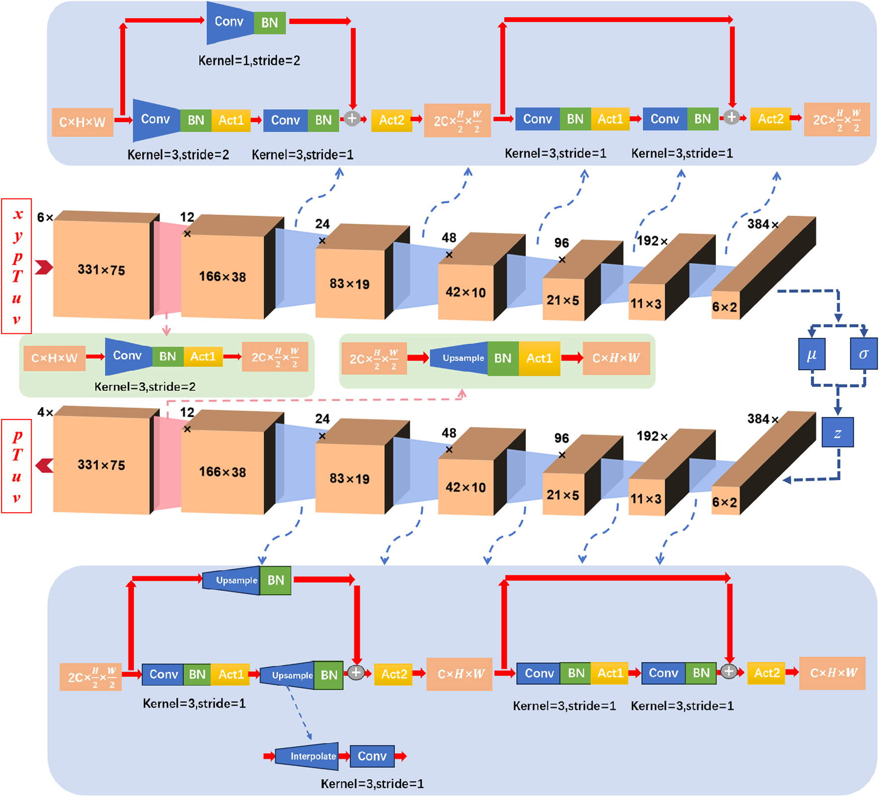
The detailed structure of VAE.
The encoder first converts 6 × 331 × 75 dimensional data to 12 × 166 × 38 dimensional data via a convolutional layer, a batch normalization layer and the LeakyReLU activation function. Considering the complex flow structures, the encoder and decoder are set up using a convolutional neural network based on ResNet [28]. The configuration ensures effective deep feature extraction without introducing redundant parameters or increasing computational complexity, thus accelerating the convergence speed of the deep network. The encoder includes five groups of ResNet modules, each comprising two residual blocks, as shown in the blue modules of the encoder in Figure 8. The feature map size is halved to achieve downsampling by adjusting the stride and padding parameters in the convolution layers. Finally, the mean value and standard deviation are obtained through fully connected layers, and the latent variable z is sampled from the normal distribution.
The decoder is used for data reconstruction and contains five groups of ResNet modules, each with two residual blocks. “Upsample” represents upsampling, consisting of a bilinear interpolation layer (Interpolate) and convolution blocks that expand the feature map to specified dimensions. The remaining residual block definitions are similar to those in the encoder, as shown by the blue modules in the decoder part of Figure 8. Finally, the dimensional feature map is converted to dimensional reconstructed flow field image via a “Upsample” module, a batch normalization layer and the LeakyReLU activation function.
The input is denoted as q, and the output is denoted as . The difference between q and is defined by a loss function during the training of the VAE. In this study, the mean square error (MSE) is adopted as the reconstruction loss , as shown in Equation 9.
MSE increases the significance of errors through squaring, which makes it more effective in leading the direction of the gradient descent algorithm. From the network training perspective, MSE forces parameter optimization to prioritize the elimination of large errors.
In the VAE, the probability distribution of the latent variable is assumed to follow a standard Gaussian distribution, i.e., . KL divergence is often used to measure the difference between two probability distributions. Therefore, the formula for calculating KL divergence in this study is shown in Equation 10.where n represents the dimension of the latent variable, and and represent the mean value and standard deviation of each latent variable.
Therefore, the loss function of the VAE is composed of two parts, as shown in Equation 11. is the weight of the KL divergence, which is an adjustable parameter.
VAE Model Considering Physical Constraints
Physics-based information can help constrain the learning process of models, making them more consistent with the physical laws of the real world. In some cases, data may be scarce or expensive, whereas physical laws are universally applicable. By incorporating physics-based information, models can be trained with limited data, thereby reducing the dependence on large datasets. Deep learning models are often considered as “black boxes,” which makes interpreting their decision-making process challenging. Physics-based information can serve as prior knowledge to improve prediction accuracy. Particularly in scenarios with high data noise or incomplete data, physics-based information acts as a form of regularization to reduce model errors. Overfitting risks can be mitigated by incorporating physical laws or constraints, which can enhance model generalization and robustness.
The fundamental physical laws, such as the conservation of mass, Newton’s second law, and the conservation of energy, are universally valid throughout the entire flow field. Since the calculation of momentum and energy involves information about the turbulence quantities that the VAE model does not predict, only the mass conservation error is considered in this study. For each reconstructed flow field, the mass flow rate is calculated for each grid cell, and the corresponding term is added to the loss function of the VAE to minimize the mass flow imbalance. This term penalizes deviations in mass conservation, guiding the model toward physically realistic flow distributions. The values of the flow variables are stored at the cell vertices, and the flow variables are interpolated from the vertices to the cell edges to compute the mass flow rate, as shown in Figure 9.
FIGURE 9
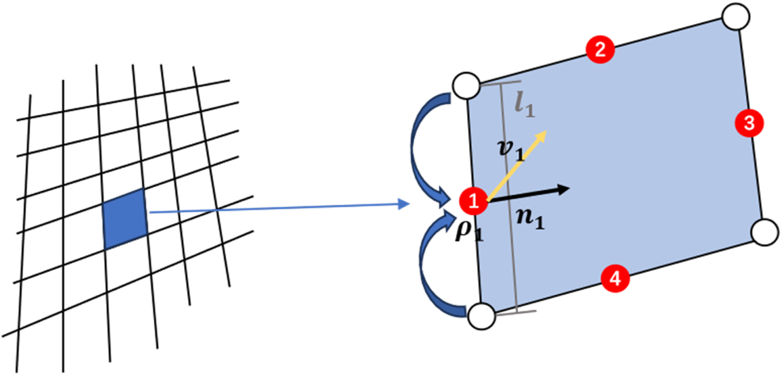
Mass flow calculation of a single cell in the 2D flow field.
Since the predicted flow field is a steady-state flow, the mass flow imbalance for each grid cell should be zero. Therefore, the mass conservation loss term is defined as shown in Equation 12, where represents the net mass flow and ij denotes the grid coordinates.
Owing to the performance of the airfoil being primarily determined by elements near the airfoil, the flow field near the airfoil is more critical than other parts of the flow field. The pressure coefficient is an important indicator for assessing the aerodynamic performance of an airfoil. Therefore, the VAE can be guided to focus more on the flow near the wall by incorporating the pressure coefficient prediction loss term into the loss function, potentially leading to better predictions of the flow field for new airfoil shapes.
The predicted value of the pressure coefficient derived from the reconstructed flow field is denoted as , and the pressure coefficient obtained from CFD calculations is denoted as . The loss term for the pressure coefficient is defined as Equation 13.
Therefore, the final form of the loss function incorporating physical constraints is shown in Equation 14, which builds on Equation 11 by adding mass conservation and pressure coefficient. is the weight of the mass conservation constraint, and is the weight of the pressure coefficient constraint, which are adjustable parameters. Properly setting the weights helps the model achieve a balanced performance between data fitting and adherence to physical laws. Specifically, excessive weight can lead to over-emphasis on the physical constraints, which may reduce data fitting accuracy. Conversely, too little weight may weaken the effect of these constraints. The detailed tuning process and the optimal weights are presented in the next section.
Training Process of VAE Model
The VAE model is implemented by PyTorch [47]. A cross-validation method is employed, which means that all the models are trained four times, and the model with the best performance on the validation set is selected. In this section, three different VAE models are trained, as shown in Figure 10. The first model (Figure 10A) is the baseline, where the loss function only includes the reconstruction loss and KL divergence. The second model (Figure 10B) incorporates the mass conservation constraint. The third model (Figure 10C) considers both mass conservation and pressure coefficient constraints. A comparison of these three models is provided at the end of this section.
FIGURE 10
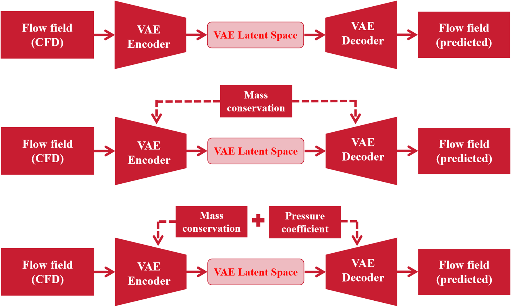
Sketch of different VAE models. (A) Baseline; (B) VAE with mass conservation; (C) VAE with mass conservation and pressure coefficient.
Training is conducted by the Adam optimizer, with an initial learning rate of 0.0001 and a batch size of 16. The learning rate is scheduled to be one-tenth of its previous value if the training set error does not decrease after two training epochs.
The physical constraints are not considered in the baseline model, which means that in the loss function of Equation 14, both and are 0. The dimension of the latent variables significantly impacts the generative capabilities of the VAE, but a higher dimension does not necessarily equal better performance. A balance between the generative effect and model complexity is needed. A high dimension might cause the model to overfit the training data, resulting in insufficient diversity in the generated samples.
KL divergence plays a crucial role in VAE, measuring the difference between the latent variable distribution and the prior distribution. In this study, the weight of KL divergence is controlled by the hyperparameter in the loss function of Equation 14, which balances the reconstruction loss and KL divergence during training. As the KL divergence weight increases, the model pays more attention to the prior distribution of the latent variable space, generating more diverse samples. The weight also affects the quality of the generated samples. Increasing the weight can generate more realistic samples. If the weight is too high, the training might be unstable, and the sample quality might be reduced. The KL divergence weight also influences the structure of the latent space, with lower weights causing more concentrated distributions and higher weights leading to more uniform or sparse distributions.
In this study, the airfoil geometry is controlled by 14 CST parameters, and the flight condition is controlled by a lift coefficient. Hence, the input is a 15-dimensional vector. Therefore, latent variable dimensions of 8, 10, 12, 14, and 16 are selected for training and testing, with KL divergence weights set in the range from to . Figure 11 shows the losses of different hyperparameters. For the same latent dimension, the reconstruction loss reaches the minimum when the KL divergence weight is . Furthermore, when the latent dimension is 12, the model demonstrates the best reconstruction performance. Figure 12 details the convergence of reconstruction loss at different latent variable dimensions when the KL divergence weight is . Intuitively, a larger latent dimension in the VAE model enhances the feature extraction capability, which can benefit flow field reconstruction. However, Figure 12 shows that larger latent dimensions also increase training difficulty, thereby reducing the reconstruction capability. Hence, selecting an appropriate latent dimension is crucial for optimal VAE model performance. In the following study, the VAE latent variable dimension is 12, and the KL divergence weight is . The total number of trainable parameters in the VAE model is 10,890,428.
FIGURE 11
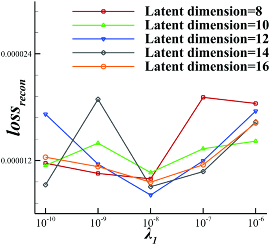
Reconstruction loss versus KL divergence weight for different latent variable dimensions.
FIGURE 12
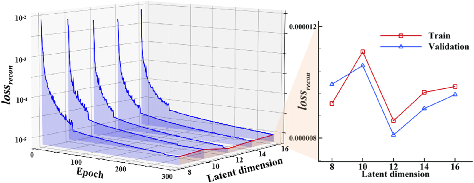
Reconstruction loss convergence of the VAE training with different latent variable dimensions for the optimal KL divergence weight.
The mass conservation constraint applies to the entire flow field. It is activated in the second model to further improve the model prediction ability, whereas the pressure coefficient constraint is not applied. Since the weights and biases in the model are randomly initialized before training begins, there is a significant difference between the reconstructed flow field and the real flow field in the early stages of training. The physical constraint loss term is large and meaningless at this stage. Enabling the physical constraints too early can cause the model to get trapped in false local optima. Experiments also show that enabling these loss terms at the beginning of training causes the gradients to diverge during backpropagation. Therefore, the mass conservation physical constraint is enabled after 100 training epochs to allow the model to first develop a foundational data-fitting ability. The mass conservation constraint weight ranges from to , increasing tenfold each time.
Figure 13 details the reconstruction loss convergence for different mass conservation constraint weights. The larger the mass conservation physical constraint weight is, the more the model focuses on adhering to mass conservation. However, if the weight is too large, the reconstruction ability of the model may decrease. Therefore, the specific value of the weight must be chosen appropriately. The reconstruction loss is minimized when the mass conservation constraint weight is , as shown in Figure 13.
FIGURE 13
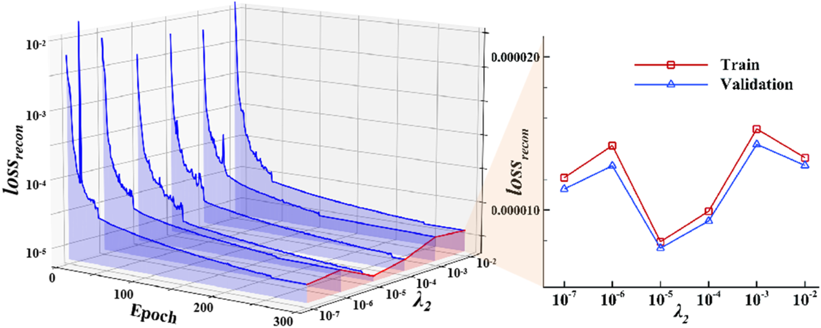
Reconstruction loss convergence of the VAE training with different mass conservation constraint weights.
The pressure coefficient constraint aims to further focus the model on the near-wall flow field. Introducing both types of physical constraints simultaneously may cause confusion during the learning process, as the model might struggle to prioritize between the mass conservation and pressure coefficient constraints. These constraints influence different regions of the flow field, and introducing them at different stages helps to ensure that the model first learns the broad principle of mass conservation across the entire flow field. This approach facilitates better learning and avoids potential conflicts in the model’s training process. Therefore, the pressure coefficient constraint is activated after 150 training epochs in the third model. The pressure coefficient physical constraint weight ranges from to , increasing tenfold each time. Figure 14 details the reconstruction loss convergence for different pressure coefficient constraint weights. Like the mass conservation constraint, the pressure coefficient constraint weight must be chosen appropriately to achieve good reconstruction performance. Figure 14 shows that the reconstruction loss is minimized when the pressure coefficient physical constraint weight is .
FIGURE 14
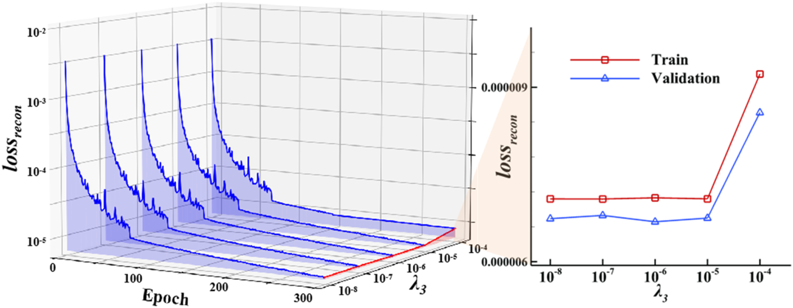
Reconstruction loss convergence of the VAE training with different pressure coefficient constraint weights.
Table 1 shows the impact of different stages of physical constraints on the VAE model’s performance. After adding the mass conservation constraint, the reconstruction loss of the VAE model decreases by 7.25%. With the additional inclusion of the pressure coefficient constraint, the reconstruction loss further decreases by 10.25%.
TABLE 1
| VAE model | Reconstruction loss | Reconstruction loss reduction |
|---|---|---|
| Baseline (without physical constraints) | 8.11 × 10⁻⁶ | -- |
| Mass conservation | 7.52 × 10⁻⁶ | 7.25% |
| Mass conservation + Pressure coefficient | 6.69 × 10⁻⁶ | 10.25% |
The impact of physical constraints on reconstruction loss.
The VAE model predicts four flow variables. The dimension of each variable is . Therefore, there are a total of 99,300 prediction points. A sample in the test set close to the mean absolute error (MAE) is selected as a typical flow field. Table 2 shows the relative error statistics of a typical flow field within different error ranges. The physical constraints effectively reduce the relative error of the prediction points, which makes them more concentrated within the 5% error range. Therefore, appropriately incorporating physical constraints helps the model adjust its learning direction, further improving its generalization ability.
TABLE 2
| Relative error | Baseline (without physical constraints) | Mass conservation | Mass conservation + Pressure coefficient |
|---|---|---|---|
| <5% | 93,902 (94.56%) | 94,113 (94.78%) | 95,769 (96.44%) |
| 5%–15% | 3,101 (3.12%) | 2,815 (2.83%) | 1,856 (1.87%) |
| 15%–50% | 1,448 (1.46%) | 1,533 (1.54%) | 842 (0.85%) |
| >50% | 849 (0.85%) | 839 (0.84%) | 833 (0.84%) |
The impact of physical constraints on the distribution of relative error.
Data Mapping Model
MLP can learn complex nonlinear relationships, which is suitable for various problems. DeepONet is a neural network architecture that is designed to learn and represent operators, which map functions to other functions. The architecture typically consists of two components: a branch network and a trunk network. The branch network processes the input function, while the trunk network processes the spatial or temporal coordinates. The outputs of these networks are then combined to produce the final output function. DeepONet can be applied to various problems, such as solving partial differential equations (PDEs), learning dynamical systems, and other tasks. It is highly flexible and can be adapted to different types of operators. In this section, DeepONet-MLP is trained and compared with the traditional MLP to demonstrate its advantages in data mapping.
After training the VAE, DeepONet-MLP is used to learn the mapping relationship between airfoil geometric CST parameters and lift coefficients to latent variables. The DeepONet-MLP framework is shown in Figure 15. The input of the network consists of 14 dimensions that describe the geometric CST parameters for the airfoil and 1 dimension for the lift coefficient, while the output is the latent variable of the VAE.
FIGURE 15

Sketch of the DeepONet-MLP model framework.
Figure 16 shows the detailed structure of different data mapping models. DeepONet-MLP has 2 parts. DeepONet comprises two subnetworks: CST net and CL net. CST net consists of 3 hidden layers, each containing 256 neurons. CL net consists of 4 hidden layers, each with 128 neurons. Layers are connected by fully connected layers and LeakyReLU activation functions. The output of CST net is a 64-dimensional vector b and r, while the output of CL net is a 64-dimensional vector w. The final output y of DeepONet is computed via the formula given in Equation 15.where i = 1, … , 64. The final 64-dimensional vector h is the output of DeepONet.
FIGURE 16
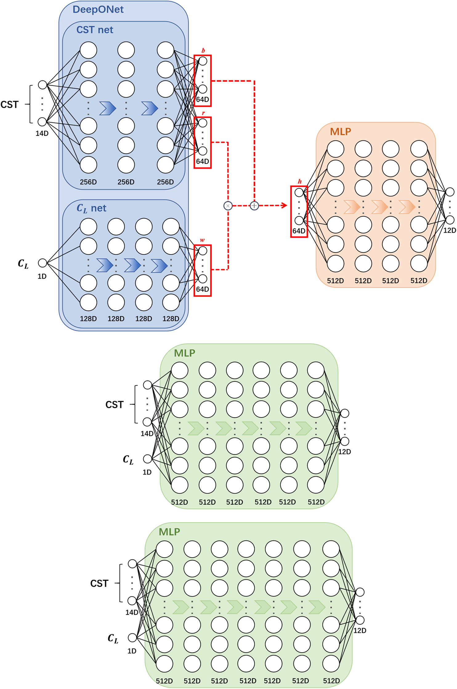
Different structures of the data mapping model (A) DeepONet-MLP; (B) MLP (6 hidden layers); (C) MLP (7 hidden layers).
In the MLP section, similar to DeepONet, layers are connected by fully connected layers and LeakyReLU activation functions. The MLP consists of 4 hidden layers, each containing 512 neurons. The output from DeepONet serves as the input for the MLP, which is then mapped to the 12-dimensional latent variable in the VAE. The DeepONet-MLP model has a total of 1,053,772 parameters.
Two simple MLPs are trained as references of the DeepONet-MLP model. Figure 16B shows the MLP model with 6 hidden layers, each containing 512 neurons. The model has a total of 1,064,972 parameters, which is similar to the DeepONet-MLP parameters. The CST parameters represent the geometric information of the airfoil, while represents the lift coefficient of the airfoil. Another MLP model with 7 hidden layers, each containing 512 neurons, has 1,327,628 parameters (Figure 16C). These 2 MLP models, with the same input and output as DeepONet-MLP, are also trained for comparison.
The loss function uses MSE, as shown in Equation 16, where n represents the dimension of the latent variable, denotes the latent variable obtained from the MLP, and z is the true value of the latent variable in the VAE.
The learning rate is scheduled to be one-tenth of its previous value if the training set error does not decrease after ten training epochs. The remainder of training settings are the same as those used for the VAE.
The training process is set for 500 epochs. Figure 17 shows the loss convergence curves of different models. Owing to the learning rate settings, all three models experience sudden decreases in loss during the training process. As shown in Table 3, with similar total trainable parameters, the DeepONet-MLP model converges to a smaller error than the MLP model with 6 hidden layers. The DeepONet-MLP model has fewer parameters and converges faster than the MLP model with 7 hidden layers with the same loss.
FIGURE 17
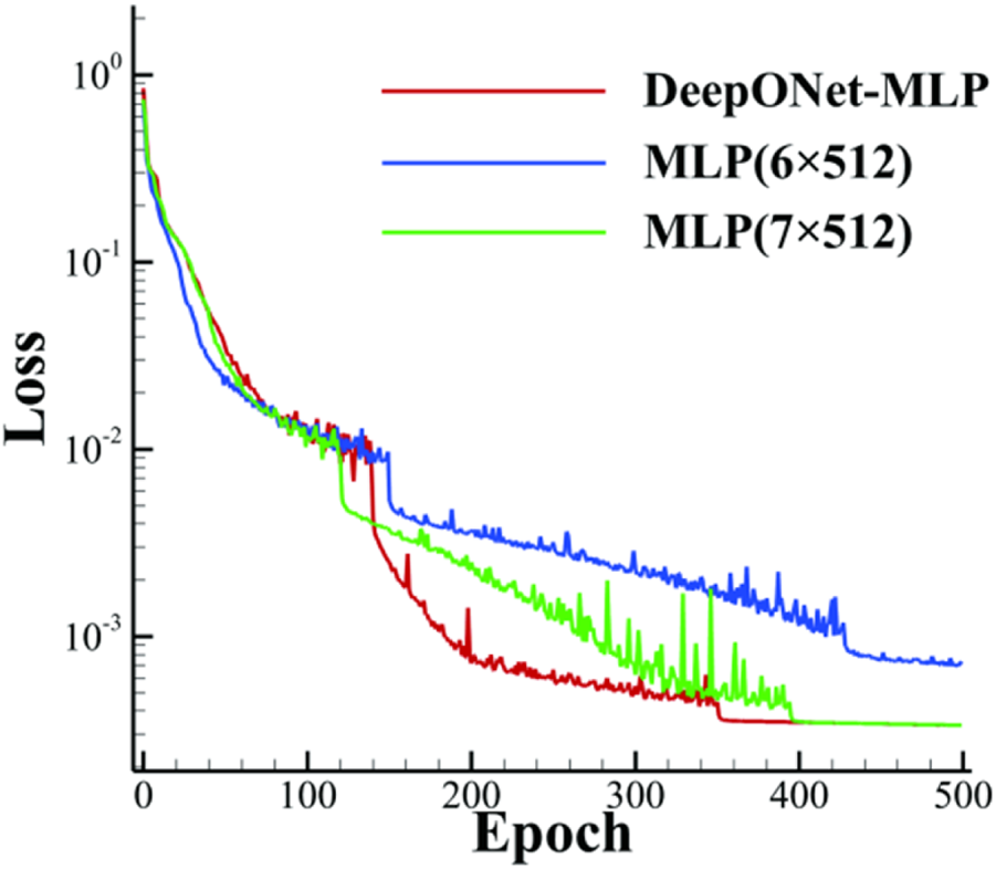
Loss convergence curves of DeepONet-MLP and MLP training.
TABLE 3
| Model Epoch | 100 | 200 | 300 | 400 | 500 | Parameters |
|---|---|---|---|---|---|---|
| DeepONet-MLP | 1.37 × 10⁻² | 7.66 × 10⁻⁴ | 5.00 × 10⁻⁴ | 3.48 × 10⁻⁴ | 3.36 × 10⁻⁴ | 1,053,772 |
| MLP(6 × 512) | 1.35 × 10⁻² | 3.65 × 10⁻³ | 2.87 × 10⁻³ | 1.18 × 10⁻³ | 7.33 × 10⁻⁴ | 1,064,972 |
| MLP(7 × 512) | 1.03 × 10⁻² | 2.27 × 10⁻³ | 7.22 × 10⁻⁴ | 3.52 × 10⁻⁴ | 3.36 × 10⁻⁴ | 1,327,628 |
Loss and parameters of DeepONet-MLP and MLP.
The MLP model processes each input parameter equally, without distinguishing between different types of inputs. However, the CST parameters are 14-dimensional, while the lift coefficient is only 1-dimensional. The disparity in dimensionality can confuse the MLP model, which lacks a mechanism to differentiate these inputs based on their physical significance. Consequently, the model might engage in inefficient learning.
Unlike a standard MLP, which treats all input parameters equally, the DeepONet model processes the CST parameters and lift coefficients by different fully connected layers. This tailored processing allows each type of input to be handled according to its characteristics, ensuring that the physical significance of each parameter is preserved and utilized effectively in the modeling process. After the inputs are individually processed, they are passed through an MLP that integrates the information to produce the final output. As a result, DeepONet-MLP is better at capturing the complex relationships between these inputs and the resulting predictions, leading to potentially higher accuracy in modeling tasks.
The distinct handling of inputs in DeepONet-MLP improves not only the model’s generalization ability but also its interpretability, as the influence of each type of input on the output can be more clearly understood. This makes DeepONet-MLP particularly advantageous in applications where understanding the contributions of different factors is crucial, such as in aerodynamic modeling.
Flow Field Prediction Results
The DeepONet-MLP-VAE model is formed by connecting the decoder in VAE with the DeepONet-MLP. The CST parameters and lift coefficient serve as the inputs for the DeepONet-MLP, which generates the corresponding latent variables. The obtained latent variables are then used as inputs to the VAE decoder to generate flow field data, completing the rapid intelligent prediction of the flow field. In Machine Learning Framework and Training Implementation, 3 different VAE models are trained: a baseline model without physical constraints, a model considering mass conservation constraints, and a model considering both mass conservation and pressure coefficient constraints. In this section, the DeepONet-MLP is connected to these 3 VAE decoders forming composite models for performance comparison, which are denoted as Model A, Model B, and Model C, as shown in Figure 18. The generalization capability of composite models is evaluated on the test dataset, which consists of data that models have not encountered during the training phase.
FIGURE 18
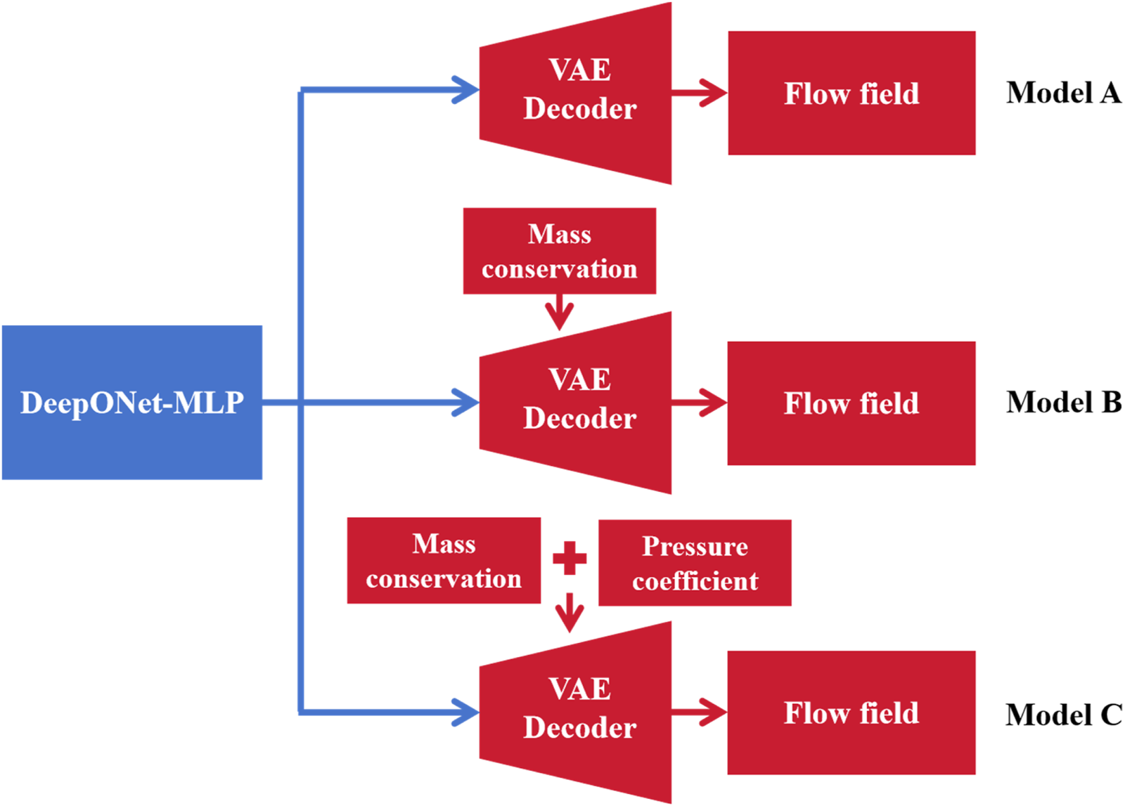
Sketch of different DeepONet-MLP-VAE models.
Four flow variables (pressure p, temperature T, velocity components u and v) of the typical flow field predicted by different composite models are shown in Figure 19. The abscissa “CFD” represents the true value gained from CFD, and the ordinate “Predict” represents the value predicted by 3 DeepONet-MLP-VAE models. The black line represents . The gray lines represent and , which represent the 5% relative error band. The scatters closer to indicate a better prediction. The statistical data indicate that 62.63% of Model A prediction points, 74.45% of Model B prediction points and 96.27% of Model C prediction points fall within the 5% relative error range. The generalization error tends to increase sharply when the DeepONet-MLP is connected to the decoder, forming a composite model. Therefore, the DeepONet-MLP-VAE, which considers both mass conservation and pressure coefficient constraints, has the best predictive performance and generalization ability after training. The generalization ability of the composite model is further improved when physical constraints are incorporated into the VAE training process.
FIGURE 19
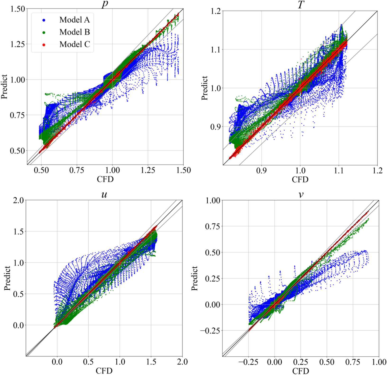
Typical sample prediction points over the test set.
Flow field contour plots and error contour plots of the typical sample are shown in Figures 20, 21. The accuracy of the 3 VAE models trained in Machine Learning Framework and Training Implementation is similar in flow field reconstruction. However, when the DeepONet-MLP is connected to the decoder in VAE, the accuracy of the composite model may decrease. The model without physical constraints loses important features of the transonic flow field. Therefore, training models solely from a data-fitting perspective makes it difficult to capture the complex transonic flow characteristics. Physical constraints can further enhance the generalization ability of composite models and help the DeepONet-MLP-VAE model better adhere to the fundamental physical laws of the real world. In shock wave regions, strong dissipation causes significant variations in the flow variables. The physical constraints enable the model to better handle the sharp gradients and extreme nonlinearity, ensuring that the predictions remain physically consistent. The flow field predicted by the DeepONet-MLP-VAE model considering both physical constraints is consistent with that of CFD, and the absolute errors are maintained within a small range.
FIGURE 20
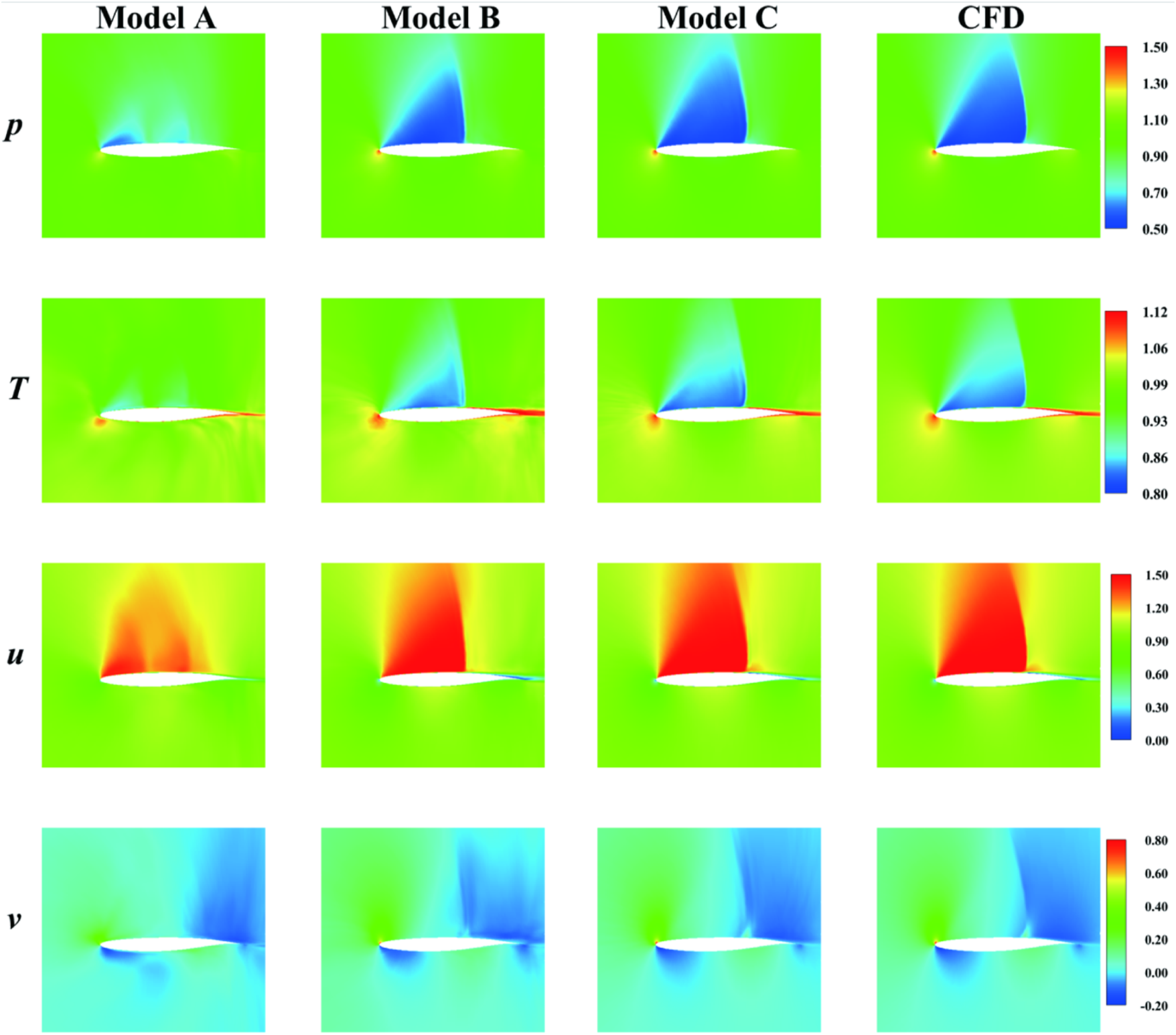
Flow field contour plots of the typical sample over the test set.
FIGURE 21
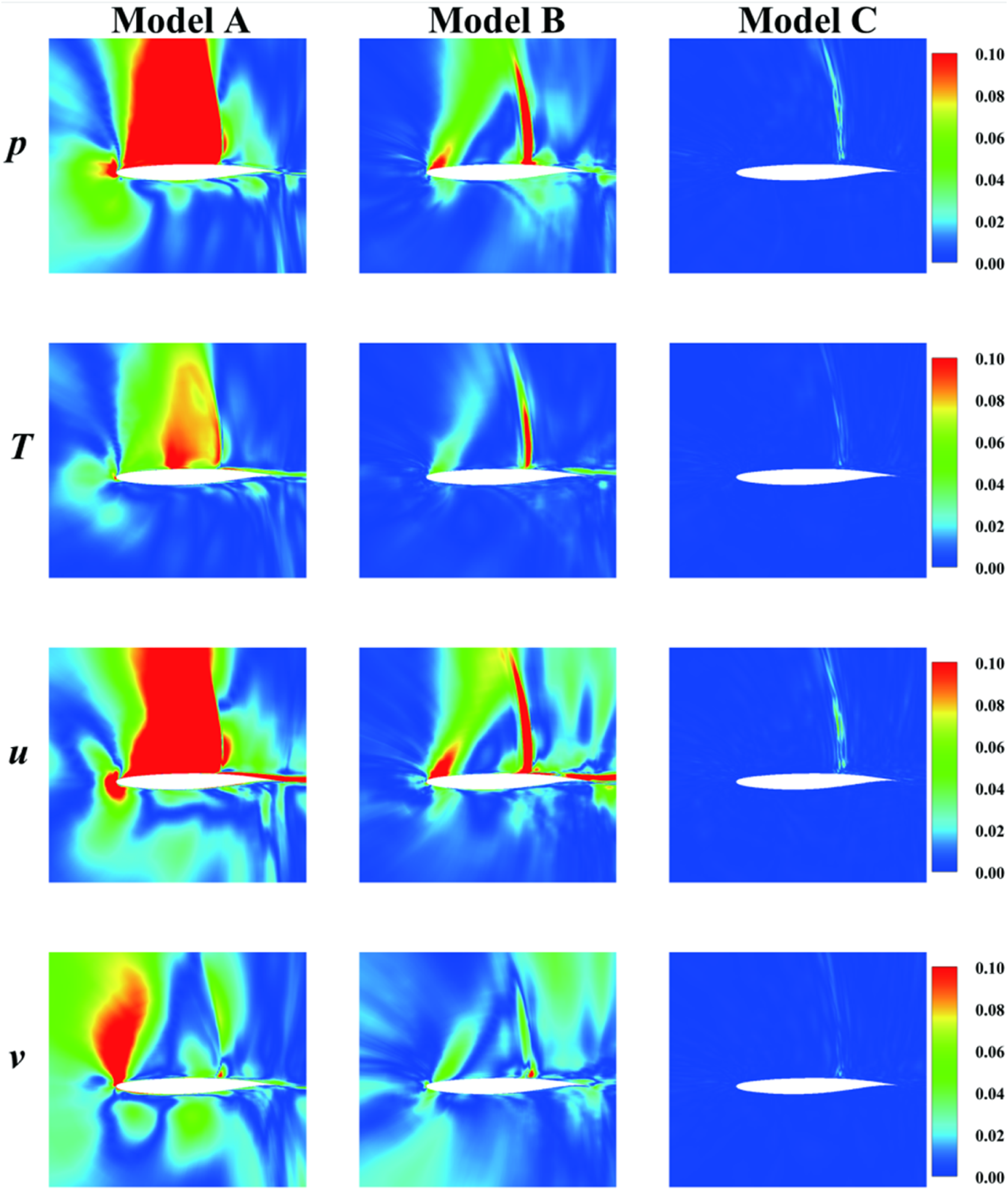
Absolute error contour plots of the typical sample over the test set.
The Cp distributions along the surface are shown in Figure 22. The velocity profiles along the surface are shown in Figure 23. The curves around the airfoil predicted by the model considering both physical constraints are almost identical to the CFD results. The pressure coefficient constraint allows the model to concentrate more on the flow characteristics near the airfoil. Consequently, the model not only better predicts Cp but also achieves better accuracy in predicting velocity profiles. Overall, the DeepONet-MLP-VAE model, which considers physical constraints, has good generalization apability and can accurately predict the flow field.
FIGURE 22
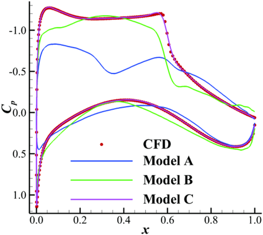
Comparison of the predicted Cp along the surface.
FIGURE 23
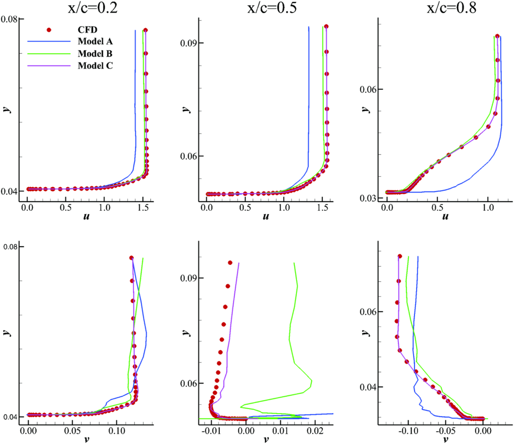
Comparison of the predicted velocity profiles along the surface.
The test set comprises 10% of the total dataset, amounting to 1,648 flow fields. Each flow field contains four flow variables. In this study, both the training and testing phases are conducted via a single computing node, each of which is configured with a 6-core CPU and one GPU. Compared with traditional CFD methods, the DeepONet-MLP-VAE model predicts flow fields at a much faster rate. Once training is complete, the model takes a total of 16.65 s to predict all the flow fields in the test set, with an average time of approximately 0.010 s per flow field, which significantly accelerates the flow field prediction process.
Conclusion
Transonic flow field prediction is crucial for supercritical airfoils, but traditional CFD methods are extremely time-consuming. This study proposes a composite DeepONet-MLP-VAE model based on deep learning, which uses airfoil geometric CST parameters and lift coefficients as inputs and generates the pressure field, temperature field, and velocity field of the airfoil, achieving rapid prediction of the flow field around supercritical airfoils. The work can be summarized as follows:
(1) By utilizing the VAE model, this study investigates the impact of latent variable dimensions and the KL divergence weight on reconstruction loss, determining the optimal parameters for feature extraction and flow field reconstruction of supercritical airfoils.
(2) The VAE training process incorporates physical constraints based on mass conservation and local physical constraints based on pressure coefficients. The appropriate incorporation of physical constraints improves model accuracy, reduces overfitting risk, and enhances model generalization ability and robustness. The results show that adding mass conservation constraints reduces reconstruction loss by 7.25%, and further adding pressure coefficient constraints reduces reconstruction loss by an additional 10.25%.
(3) By combining the structures of MLP and DeepONet, a DeepONet-MLP network with higher accuracy and fewer parameters is designed to achieve the nonlinear mapping from airfoil geometric CST parameters and lift coefficients to latent variables in the VAE. The DeepONet-MLP-VAE composite model can accurately and efficiently predict the flow field around supercritical airfoils, including accurate predictions in shock wave regions.
The proposed DeepONet-MLP-VAE composite model, which incorporates multiple physical constraints during training, offers a valuable and promising method for rapid flow field prediction and reconstruction of transonic flow fields around supercritical airfoils. Extending the DeepONet-MLP-VAE model to the prediction of 3D flow fields for wings will be carried out in subsequent research.
Statements
Data availability statement
Publicly available datasets were analyzed in this study. This data can be found here: https://github.com/YangYunjia/floGen.
Author contributions
ML participated in the study design, programming, surrogate model training, data analysis, plotting, and manuscript writing. YnY provided the airfoil flow field dataset and offered insights on the VAE training. CW contributed improvement suggestions for the DeepONet model. YZ was responsible for manuscript review, editing, and provided valuable suggestions on the article structure and figure creation. All authors contributed to the article and approved the submitted version.
Funding
The author(s) declare that financial support was received for the research, authorship, and/or publication of this article. This work was supported by the National Natural Science Foundation of China (Grant Nos U23A2069, 12372288, 12388101, and 92152301).
Acknowledgments
The authors would like to thank Gongyan Liu and Weishao Tang for their inspiring comments on the work.
Conflict of interest
The authors declare that the research was conducted in the absence of any commercial or financial relationships that could be construed as a potential conflict of interest.
Generative AI statement
The author(s) declare that no Generative AI was used in the creation of this manuscript.
References
1.
LiJHeSMartinsJRRA. Data-driven Constraint Approach to Ensure Low-Speed Performance in Transonic Aerodynamic Shape Optimization. Aerospace Sci Technology (2019) 92:536–50. 10.1016/j.ast.2019.06.008
2.
BuckleyHPZhouBYZinggDW. Airfoil Optimization Using Practical Aerodynamic Design Requirements. J Aircraft (2010) 47(5):1707–19. 10.2514/1.c000256
3.
RamyaPKumarAHMoturiJRamanaiahN. Analysis of Flow Over Passenger Cars Using Computational Fluid Dynamics. Int J Eng Trends Technology (Ijett) (2015) 29:170–6. 10.14445/22315381/ijett-v29p232
4.
ZhangHDaiLXuGLiYChenWTaoWQ. Studies of Air-Flow and Temperature Fields inside a Passenger Compartment for Improving Thermal Comfort and Saving Energy. Part I: Test/numerical Model and Validation. Appl Therm Eng (2009) 29(10):2022–7. 10.1016/j.applthermaleng.2008.10.005
5.
SkamarockWCKlempJB. A Time-Split Nonhydrostatic Atmospheric Model for Weather Research and Forecasting Applications. J Comput Phys (2008) 227(7):3465–85. 10.1016/j.jcp.2007.01.037
6.
NigamPKTenguriaNPradhanMK. Analysis of Horizontal Axis Wind Turbine Blade Using CFD. Int J Eng Sci Technology (2017) 9(2):46–60. 10.4314/ijest.v9i2.5
7.
TrivediCCervantesMJGunnar DahlhaugO. Numerical Techniques Applied to Hydraulic Turbines: A Perspective Review. Appl Mech Rev (2016) 68(1):010802. 10.1115/1.4032681
8.
ChoiCRKimCN. Numerical Investigation on the Flow, Combustion and NOx Emission Characteristics in a 500 MWe Tangentially Fired Pulverized-Coal Boiler. Fuel (2009) 88(9):1720–31. 10.1016/j.fuel.2009.04.001
9.
HatamiMJafaryarMGanjiDDGorji-BandpyM. Optimization of Finned-Tube Heat Exchangers for Diesel Exhaust Waste Heat Recovery Using CFD and CCD Techniques. Int Commun Heat Mass Transfer (2014) 57:254–63. 10.1016/j.icheatmasstransfer.2014.08.015
10.
SalimSMBuccolieriRChanADi SabatinoS. Numerical Simulation of Atmospheric Pollutant Dispersion in an Urban Street Canyon: Comparison between RANS and LES. J Wind Eng Ind Aerodynamics (2011) 99(2-3):103–13. 10.1016/j.jweia.2010.12.002
11.
HarrisCD. NASA Supercritical Airfoils: A Matrix of Family-Related Airfoils. (1990).
12.
NakayamaA. Characteristics of the Flow Around Conventional and Supercritical Airfoils. J Fluid Mech (1985) 160:155–79. 10.1017/s0022112085003433
13.
HurleyFXSpaidFWRoosFWStiversL. SBandettiniA. Detailed Transonic Flow Field Measurements about a Supercritical Airfoil Section. (1975).
14.
LiemRPMaderCAMartinsJRRA, Surrogate Models and Mixtures of Experts in Aerodynamic Performance Prediction for Aircraft Mission Analysis. Aerospace Sci Technology (2015) 43:126–51. 10.1016/j.ast.2015.02.019
15.
GunnSR. Support Vector Machines for Classification and Regression. ISIS Tech Rep (1998) 14(1):5–16.
16.
PanLHeCTianYWangHZhangXJinY. A Classification-Based Surrogate-Assisted Evolutionary Algorithm for Expensive Many-Objective Optimization. IEEE Trans Evol Comput (2018) 23(1):74–88. 10.1109/tevc.2018.2802784
17.
LeifssonLTKozielSHosderS. Multi-objective Aeroacoustic Shape Optimization by Variable-Fidelity Models and Response Surface Surrogates. In: Structural Dynamics, and Materials Conference (2015). 1800.
18.
RenganathanSAMaulikRAhujaJ. Enhanced Data Efficiency Using Deep Neural Networks and Gaussian Processes for Aerodynamic Design Optimization. Aerospace Sci Technology (2021) 111:106522. 10.1016/j.ast.2021.106522
19.
BrahmacharySBhagyarajanAOgawaH. Fast Estimation of Internal Flowfields in Scramjet Intakes via Reduced-Order Modeling and Machine Learning. Phys Fluids (2021) 33(10). 10.1063/5.0064724
20.
RaissiMWangZTriantafyllouMSKarniadakisGE. Deep Learning of Vortex-Induced Vibrations. J Fluid Mech (2019) 861:119–37. 10.1017/jfm.2018.872
21.
WuHLiuXAnWChenSLyuH. A Deep Learning Approach for Efficiently and Accurately Evaluating the Flow Field of Supercritical Airfoils. Comput & Fluids (2020) 198:104393. 10.1016/j.compfluid.2019.104393
22.
DuXHePMartinsJRRA. Rapid Airfoil Design Optimization via Neural Networks-Based Parameterization and Surrogate Modeling. Aerospace Sci Technology (2021) 113:106701. 10.1016/j.ast.2021.106701
23.
LuLJinPPangGZhangZKarniadakisGE. Learning Nonlinear Operators via DeepONet Based on the Universal Approximation Theorem of Operators. Nat machine intelligence (2021) 3(3):218–29. 10.1038/s42256-021-00302-5
24.
RumelhartDEHintonGEWilliamsRJ. Learning Representations by Back-Propagating Errors. nature (1986) 323(6088):533–6. 10.1038/323533a0
25.
KingmaDPWellingM. Auto-encoding Variational Bayes. arXiv preprint arXiv:1312.6114 (2013).
26.
LiRZhangYChenH. Mesh-Agnostic Decoders for Supercritical Airfoil Prediction and Inverse Design. arXiv preprint arXiv:2402.17299 (2024) 62:2144–60. 10.2514/1.j063387
27.
SohnKLeeHYanX. Learning Structured Output Representation Using Deep Conditional Generative Models. Adv Neural Inf Process Syst (2015) 28.
28.
HeKZhangXRenSSunJDeep Residual Learning for Image recognition. in: Proceedings of the IEEE Conference on Computer Vision and Pattern Recognition (2016). 770–8.
29.
DengKChenHZhangY. Flow Structure Oriented Optimization Aided by Deep Neural Network. in: 10th International Conference on Computational Fluid Dynamics (ICCFD10). (2018).
30.
SekarVJiangQShuCKhooBC. Fast Flow Field Prediction Over Airfoils Using Deep Learning Approach. Phys Fluids (2019) 31(5). 10.1063/1.5094943
31.
WangJHeCLiRChenHZhaiCZhangM. Flow Field Prediction of Supercritical Airfoils via Variational Autoencoder Based Deep Learning Framework. Phys Fluids (2021) 33(8). 10.1063/5.0053979
32.
DuboisPGomezTPlanckaertLPerretL. Machine Learning for Fluid Flow Reconstruction from Limited Measurements. J Comput Phys (2022) 448:110733. 10.1016/j.jcp.2021.110733
33.
LiRZhangYChenH. Physically Interpretable Feature Learning of Supercritical Airfoils Based on Variational Autoencoders. AIAA J (2022) 60(11):6168–82. 10.2514/1.j061673
34.
YangYLiRZhangYChenH. Flowfield Prediction of Airfoil Off-Design Conditions Based on a Modified Variational Autoencoder. AIAA J (2022) 60(10):5805–20. 10.2514/1.j061972
35.
ChenDGaoXXuCWangSChenSFangJet alFlowDNN: A Physics-Informed Deep Neural Network for Fast and Accurate Flow Prediction. Front Inf Technology & Electron Eng (2022) 23(2):207–19. 10.1631/fitee.2000435
36.
DuruCAlemdarHBaranOU. A Deep Learning Approach for the Transonic Flow Field Predictions Around Airfoils. Comput & Fluids (2022) 236:105312. 10.1016/j.compfluid.2022.105312
37.
TanZLiRZhangY. Flow Field Reconstruction of 2D Hypersonic Inlets Based on a Variational Autoencoder. Aerospace (2023) 10(9):825. 10.3390/aerospace10090825
38.
LiuGLiRZhouXSunTZhangY. Reconstruction and Fast Prediction of 3D Heat and Mass Transfer Based on a Variational Autoencoder. Int Commun Heat Mass Transfer (2023) 149:107112. 10.1016/j.icheatmasstransfer.2023.107112
39.
KulfanBBussolettiJ. Fundamental Parameteric Geometry Representations for Aircraft Component shapes. In: 11th AIAA/ISSMO Multidisciplinary Analysis and Optimization Conference (2006). p. 6948.
40.
KulfanBM. Universal Parametric Geometry Representation Method. J aircraft (2008) 45(1):142–58. 10.2514/1.29958
41.
RunzeLZhangYHaixinC. Pressure Distribution Feature-Oriented Sampling for Statistical Analysis of Supercritical Airfoil Aerodynamics. Chin J Aeronautics (2022) 35(4):134–47.
42.
WhiteJ. Elliptic Grid Generation with Orthogonality and Spacing Control on an Arbitrary Number of Boundaries[C]//21st Fluid Dynamics. In: Plasma Dynamics and Lasers Conference (1990). p. 1568.
43.
KristSLBiedronRTRumseyCL. CFL3D User’s Manual (Version 5.0),. NASA/TM-1998–208444 (1998).
44.
JacquinLMoltonPDeckSMauryBSoulevantD. Experimental Study of Shock Oscillation over a Transonic Supercritical Profile. AIAA J (2009) 47(9):1985–94. 10.2514/1.30190
45.
TranDRanganathRBleiDM. The Variational Gaussian Process. arXiv preprint arXiv:1511.06499 (2015).
46.
DubeyAKJainV. Comparative Study of Convolution Neural Network’s Relu and Leaky-Relu Activation Functions. In: Applications of Computing Automation and Wireless Systems in Electrical Engineering: Proceedings of MARC 2018. Singapore: Springer (2019). p. 873–80.
47.
PaszkeAGrossSMassaFLererABradburyJChananGet alPytorch: An Imperative Style, High-Performance Deep Learning Library. Adv Neural Inf Process Syst (2019) 32.
Summary
Keywords
fast flow field prediction, supercritical airfoils, variational autoencoder, deep operator network, physical constraints
Citation
Liu M, Yang Y, Wu C and Zhang Y (2024) A Fast Prediction Model of Supercritical Airfoils Based on Deep Operator Network and Variational Autoencoder Considering Physical Constraints. Aerosp. Res. Commun. 2:13901. doi: 10.3389/arc.2024.13901
Received
08 October 2024
Accepted
27 November 2024
Published
20 December 2024
Volume
2 - 2024
Updates
Copyright
© 2024 Liu, Yang, Wu and Zhang.
This is an open-access article distributed under the terms of the Creative Commons Attribution License (CC BY). The use, distribution or reproduction in other forums is permitted, provided the original author(s) and the copyright owner(s) are credited and that the original publication in this journal is cited, in accordance with accepted academic practice. No use, distribution or reproduction is permitted which does not comply with these terms.
*Correspondence: Yufei Zhang, zhangyufei@tsinghua.edu.cn
Disclaimer
All claims expressed in this article are solely those of the authors and do not necessarily represent those of their affiliated organizations, or those of the publisher, the editors and the reviewers. Any product that may be evaluated in this article or claim that may be made by its manufacturer is not guaranteed or endorsed by the publisher.